Week 2 Air standard Cycle

Air standard cycle – Otto cycle (report)

The whole program can be subdivided into 13 subcategories.

• Input variables to the program: Here the input variable such as the temperature of the fluid mixture after combustion namely T3 and the gamma value for air are specified.

The inputs were as follows,

T3 = 2300K

T1 = 500K

Gamma (air) = 1.4

• Specifying state point 1 variables: The state point variable at point 1 namely P1, V1, and T1 are to be specified.

P1 is assumed to be atmospheric pressure of 1 bar.

An initial temperature of 500 Kelvin is assumed before the compression process T1.

• In order to get the V1 and V2 values, geometric parameters of the engine are considered such as

Bore = 0.1m

Stroke = 0.1m

Connecting rod, con_rod = 0.15m

Compression ratio, cr = 8

• From the geometric parameters,

Swept volume is calculated as v_swept = (pi/4)*bore^2*stroke

Clearance volume is calculated as v_clearance = v_swept/(cr-1)

From the above relations,

V1= v_swept + v_clearance

V2= v_clearance

• State variables at point 2

Pressure at point 2 can be obtained from the isentropic relation

P2= P1*cr^gamma

The temperature at point 2 can be obtained from the ideal gas equation (P*V)/T=constant

T2=p2*v2*T1/(p1*v1)

• Calculation of residual volume for the compression stroke

The isentropic constant is first calculated from the isentropic relation,

P1*V1^gamma=constant_1

Subsequently, a function is called named ‘engine_kinematics’ which gives back the volume trace at each value of theta from 180 to 0 degrees (compression stroke), this value is stored in the variable named V_compression

• Pressure calculation corresponding to the values stored in V_compression

The pressure at each point during the compression stroke is calculated as per the code

P_compression.append(constant/pow(v,gamma))

This is basically the modified form of the equation P*V^gamma = constant

• Calculating state variable at point 3

Since 2-3 is a constant volume heat addition process, V3=V2

P3 is obtained from the ideal gas equation, p3=p2*T3/T2

• State variables at point 4

Since 4-1 is a constant volume heat rejection process, V4=V1

P4 can be calculated using the isentropic relation P*V^gamma= constant,

p4=p3*(v3/v4)^gamma

• Calculation of residual volume for expansion stroke

The isentropic constant is first calculated from the isentropic relation,

P2*V2^gamma=constant_2

Subsequently, a function is called named ‘engine_kinematics’ which gives back the volume trace at each value of theta from 0 to 180 degrees (expansion stroke), this value is stored in the variable named V_expansion

• Pressure calculation corresponding to the values stored in V_expansion

The pressure at each point during the expansion stroke is calculated as per the code

P_expansion.append(constant/pow(v,gamma))

This is basically the modified form of the equation P*V^gamma = constant

• Plotting the graph

Points 1,2,3 and 4 are plotted using different variations of the command such as

#plotting code
plt.plot([v2, v3],[ p2, p3])
plt.plot(V_compression, P_compression)
plt.plot(V_expansion, P_expansion)
plt.plot([v4, v1],[ p4, p1])
plt.xlabel('Volume in m^3')
plt.ylabel('Pressure in Pascal')
plt.show()
eff = 1-pow((v2/v1),(gamma-1))

Subsequently, the figure is given a label and the axes are specified using the commands,

plt.xlabel(‘…’)

plt.ylabel(‘…’)

• Calculating the efficiency of the cycle

The efficiency of the cycle can be calculated from the equation,

efficiciency = 1- (v2/v1)^(gamma-1)

and for this example, it was found to be 0.564

• Description of the function ‘engine_kinematics’

Code: def engine_kinematics(bore, stroke, con_rod, cr, start_crank, end_crank):

As per the code the function takes is 6 values during the function call namely bore diameter, stroke length, connecting rod length, compression ratio, start crank angle and end crank angle.

Inside the function the crank pin radius a, R value, swept volume v_s and clearance volume v_c is specified as per the code,

v_s = pi/4*bore^2*stroke;

v_c = v_s/(cr-1);

Various values of theta are obtained from the linspace command for compression and expansion.

The trace volume is calculated from the equation

V = (1 + term1*(term2 - term3))*v_c

Where term1,2 and 3 are given as

term1 =0.5*(cr-1);

term2 = R +1 - cos(theta);

term3 = (R^2 -sin(theta)^2)^0.5;

Main Program

import matplotlib.pyplot as plt
import math
import numpy as np


#function for determining the volume trace from compression and expansion
def engine_kinematics(bore, stroke, con_rod, cr, start_crank, end_crank):
	
	#geometric parameters
	a = stroke/2 #crank pin radius
	R = con_rod/a 


	#volume parameters
	V_s = math.pi*(1/4)*pow(bore,2)*stroke #swept volume
	V_c = V_s/(cr-1) #clearance volume

	V=[]


	sc = math.radians(start_crank)  #start crank angle
	ec = math.radians(end_crank)   # end crank angle

	num_values = 50 #number of traces required
	theta = np.linspace(sc,ec,num_values) #creating the required crank angle values


# calculation for volume trace
	for th in theta:
		term1 = 0.5*(cr-1)
		term2 = R + 1 - math.cos(th)
		term3 = pow(pow(R,2) - pow(math.sin(th),2),0.5)

		V.append((1+ term1*(term2 - term3))*V_c)


	return V


#inputs
p1 = 101325
t1 = 500 
gamma = 1.4

#geometric parameters
bore = 0.1
stroke = 0.1
con_rod = 0.15
cr = 8
t3 = 2300 # assumed temperature at constant volume heat addition process

#volume computation
v_s = (math.pi/4)*pow(bore,2)*stroke
v_c = v_s/(cr-1)
v1 = v_c + v_s


#state point 2
v2 = v_c

#p2v2^gamma = p1v1^gamma
p2 = p1*pow(v1,gamma)/pow(v2,gamma)


#p2v2/t2 = p1v1/t1 | rhs = p1v1/t1 | rhs = p2v2/t2 | t2 = p2v2/rhs
rhs =p1*v1/t1
t2 = (p2*v2)/rhs
V_compression = engine_kinematics(bore, stroke, con_rod, cr, 180, 0)

constant = p1*pow(v1,gamma)

#calculation of pressure values for corresponding volume during compression
P_compression = []

for v in V_compression:
	P_compression.append(constant/pow(v,gamma))



#state pint point 3
v3 = v2 #constant volume heat addition process

#p3v3/t3 = p2v2/t2 | rhs = p2v2/t2 | p3 = rhs*t3/v3

rhs = p2*v2/t2
p3 = rhs*t3/v3


V_expansion = engine_kinematics(bore, stroke, con_rod, cr, 0, 180)

constant = p3*pow(v3,gamma)


#calculation of pressure values for corresponding volume during expansion
P_expansion = []

for v in V_expansion:
	P_expansion.append(constant/pow(v,gamma))

#state point 4

v4 = v1

#p4v4^gamma = p3v3^gamma

p4 = p3*pow(v3,gamma)/pow(v4,gamma)

#p4v4/t4 = p3v3/t3 = rhs | rhs is constant for a closed system
t4 = p4*v4/rhs

#plotting code
plt.plot([v2, v3],[ p2, p3])
plt.plot(V_compression, P_compression)
plt.plot(V_expansion, P_expansion)
plt.plot([v4, v1],[ p4, p1])
plt.xlabel('Volume in m^3')
plt.ylabel('Pressure in Pascal')
plt.show()
eff = 1-pow((v2/v1),(gamma-1))
print('efficiency =',str(eff))

Outputs:

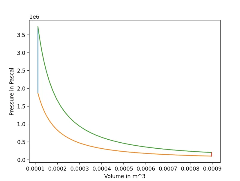Figure 1: PV diagram

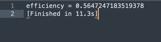
Figure 2: Output showing Efficiency of cycle