Hacker Statistics approach for finding the probability distribution of a die game.

Problem statement: To find the probability distribution of reaching 60 or greater steps at the end of 100 die throws.

Game explanation: A die is thrown 100 times and steps are taken as per the following instructions

The player first throws the die:

• If the number of eyes on the die is 1 or 2 the player should take 1 step back.
• If the number of eyes on the die is 3, 4 or 5 the player should take 1 step forward.
• If the number of eyes on the die is 6 the player throws the die again and takes the number of steps corresponding to the number on the die thrown the second time.

Additional rules:

• The player cannot go below step 0.
• There is always a 0.1% chance of the player falling down to step 0 with every throw.

Solution method selection:

Since the analytical approach for the solution to this problem is somewhat complex, we take another approach.

We take the number of steps in each throw as a 'random step' and such steps are appended after each throw to create a 'random walk'. Several such walks are simulated and the resulting data is analysed. This methodology is called the Hacker Statistics approach.

Program to simulate 10 random walks w/o a chance of falling

# numpy and matplotlib imported, seed set.

# initialize and populate all_walks
all_walks = []
for i in range(10) :
    random_walk = [0]
    for x in range(100) :
        step = random_walk[-1]
        dice = np.random.randint(1,7)
        if dice <= 2:
            step = max(0, step - 1)
        elif dice <= 5:
            step = step + 1
        else:
            step = step + np.random.randint(1,7)
        random_walk.append(step)
    all_walks.append(random_walk)

# Convert all_walks to NumPy array: np_aw
np_aw = np.array(all_walks)

# Plot np_aw and show
plt.plot(np_aw)
plt.show()

# Clear the figure
plt.clf()

# Transpose np_aw: np_aw_t
np_aw_t = np.transpose(np_aw)

# Plot np_aw_t and show
plt.plot(np_aw_t)
plt.xlabel('Number of throws')
plt.ylabel('Step number')
plt.show()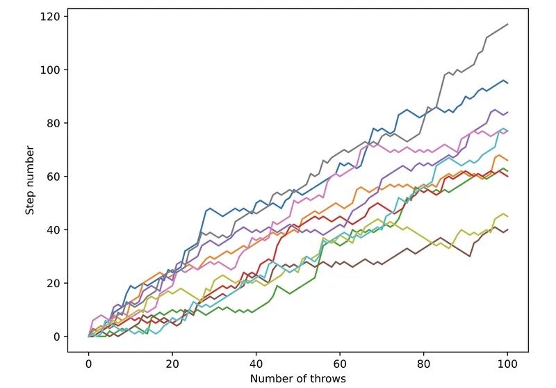

Program to simulate 10 random walks with 0.1% chance of falling

# numpy and matplotlib imported, seed set

# Simulate random walk 250 times
all_walks = []
for i in range(10) :
    random_walk = [0]
    for x in range(100) :
        step = random_walk[-1]
        dice = np.random.randint(1,7)
        if dice <= 2:
            step = max(0, step - 1)
        elif dice <= 5:
            step = step + 1
        else:
            step = step + np.random.randint(1,7)

        # Implement clumsiness
        if np.random.rand() < 0.001 :
            step = 0

        random_walk.append(step)
    all_walks.append(random_walk)

# Create and plot np_aw_t
np_aw_t = np.transpose(np.array(all_walks))
plt.plot(np_aw_t)
plt.xlabel('Number of Throws')
plt.ylabel('Step Number')
plt.show()
plt.clf()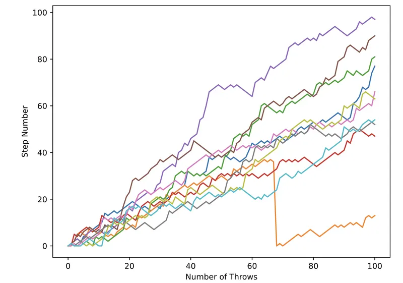

Program to calculate the distribution for 500 simulations

# numpy and matplotlib imported, seed set

# Simulate random walk 500 times
all_walks = []
for i in range(500) :
    random_walk = [0]
    for x in range(100) :
        step = random_walk[-1]
        dice = np.random.randint(1,7)
        if dice <= 2:
            step = max(0, step - 1)
        elif dice <= 5:
            step = step + 1
        else:
            step = step + np.random.randint(1,7)
        if np.random.rand() <= 0.001 :
            step = 0
        random_walk.append(step)
    all_walks.append(random_walk)

# Create and plot np_aw_t
np_aw_t = np.transpose(np.array(all_walks))

# Select last row from np_aw_t: ends
ends = np.array(np_aw_t[-1,:])

# Plot histogram of ends, display plot
plt.hist(ends, alpha = 0.5)
plt.xlabel('Number of steps')
plt.ylabel('# of hits for correspoding steps')
plt.show()
# plt.clf()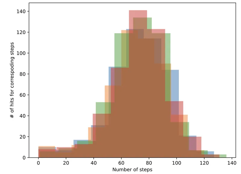

The probability distribution for 500 simulations was then plotted. It becomes clear with an increasing number of simulations that we get a distributed bell curve.

From the data obtained for 500 simulations, the probability of getting at least 60 steps was calculated to be 78.4% which is quite high. So the player has a high chance of winning this bet.