Week 3 - Solving second order ODEs

Week 3 Challenge, Solving second-order ODEs and animating a simple pendulum

Report:

The program starts with providing input data for the simple pendulum such as damping coefficient, the mass of the ball, acceleration due to gravity and length of the pendulum.

The following inputs were provided,

Damping coefficient, b = 0.05

Mass of the ball, m = 1 kg

Acceleration due to gravity, g = 9.81 m/s^2

Length of the pendulum, l = 1 m

The initial condition for the ODE was specified next,

Starting displacement = 0 rad

Initial angular velocity = 3 rad/s

The ODE was solved for a time span ranging from 0-20 seconds as specified in the input code for the variable t.

Next, the ODE was solved by calling the odeint solver with the independent variables t and theta and by passing the function ‘ode_solve’ with the input variables t, theta_0, b, n, g and l.

Furthermore, the integration span ‘t was specified with the initial condition stored in the variable ‘theta_0’.

Code for animation was specified next.

The fixed points for the pendulum were specified with the coordinates x_0 and y_0.

Each still of the plot was made using plot commands. subsequently, a movie was made using an online gif maker

Inside the function ‘ode_solve’,

The second-order ODE was simplified into a system of first-order ODEs, solved and sent back to the main program.

Main Program:

import matplotlib.pyplot as plt
import math
import numpy as np
from scipy.integrate import odeint




# functions for solving ODE
def ode_solve (theta,t,b,g,l,m):
	tht1 = theta[0]
	tht2 = theta[1]
	d_tht1 = tht2
	d_tht2 = -(b/m)*tht2 - (g/l)*math.sin(tht1)
	d_tht = [d_tht1, d_tht2]
	return d_tht

#entering input parameters
l = 1
m = 1
b = 0.05
g = 9.81

#time span
t = np.linspace(0,20,200)

#initial condition
theta_0 = [0, 3]

#solbing ODE
theta = odeint(ode_solve, theta_0, t, args = (b,g,l,m))


#plotting results
plt.plot(t,theta[:,0])
plt.plot(t,theta[:,1])
plt.xlabel('time')
plt.ylabel('plot')
plt.show()


#making figures for animation
x0 = 0
y0 = 0
ct = 1

for t in theta[:,0]:


	x1 = l*math.sin(t) 
	y1 = -l*math.cos(t) # negative value for inverting the pendulum downwards
	filename = str(ct) + '.jpg'
	ct += 1

	plt.figure()
	plt.plot([-0.7, 0.7], [0, 0], 'black', linewidth = 3) #plotting base of the pendulum
	plt.plot([x0, x1], [y0, y1], 'red', linewidth = 2 ) #plotting the string
	plt.plot(x0,y0, 'o', markersize = 4) #plotting the base of the pendulum
	plt.plot(x1,y1, 'o', markersize = 10) #plotting the bob of the pendulum
	plt.xlim([-1.5, 1.5]) #defining x limit
	plt.ylim([-1.5, 1.5]) #defining y limit
	plt.title('Animation of simple pendulum')
	plt.savefig(filename)

Outputs:

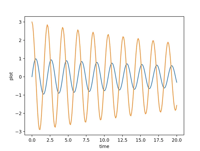
Figure 1: variation of velocity and displacement of the bob of a pendulum with time

Animation file : https://drive.google.com/file/d/14I-qVtVSXtmlD83Q1S4ucyK__XCyiJ5j/view?usp=sharing