PYTHON Week 5 - Curve fitting
WEEK 5: CURVE FITTING
AIM
Write a code for fit linear and cubic polynomial curves in python programming.
OBJECTIVE
The main objective is to understand the curve fitting and write the code for the linear curve and cubic polynomial curve and plot the graph with data points
Also, measure the fitness characteristics for both the curves
The code is written for this need to be as popt, pcov wat is the use of them for the output of the curve fit.
THEORY
Curve Fitting is the process to construct the curve or mathematical function that has been best fit to data points, which is possible to subject to constraints. curve fitting can be involved as interpolation, where an exact fit to the data is required, or smoothing in which smooth function is constructed that approximately fits the data.
Linear curve fitting, in this a linear curve is a that has linear independence on the curve parameters. Examples of the linear curve lines, polynomials, Chebyshev series, and any linear combination of a set of curves. The linearity simplifies the calculations, as the solution can be expressed in terms of simple linear algebra.
Most curve fitting is done in linear combinations of a set of basis functions. A linear combination a set of function f1, f2....., fn is a function whose value is given by:
f(x) = a1f1(x) + a2f2(x) + ... + anfn(x)
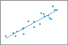
Fig 1: Linear curve fitting
The cubic polynomial curve is the curve when we fit our data to the graph of the polynomial function. The same least-squares method can be used to find the polynomial, of a given degree, that has the minimum total error.
To choose the best fit for the curve the following four parameters help us to measure the goodness of fit criteria or how well the equations are representing the given data points:
- Sum of squares due to the error (SSE).
- R-square (R2)
- Adjusted R-square
- Root mean squared error (RMSE)
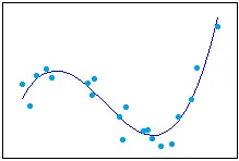
Fig 2: Cubic curve
PROCEDURE
- Importing the numpy, matplotlib, and scipy to plot result and output the data value.
- For curve fitting, output these two functions are defined as linear and cubical.
- To define the linear curve function following code is written: # Curve_fit function for linear polynomial
def func(t, a, b):
return a*t + b - And for the cubic polynomial curve: # Curve_fit function for cubical polynomial
def func_1(t, a, b, c, d):
return a*pow (t,3) + b*pow(t,2) + c*t +d - After defining the function the data value of temperature to read as provided defining the read file with temperature and cp in the null array, for line in open('data', 'r'):
values = line.split(',')
temperature.append(float(values[0]))
cp.append(float(values[1])) and then returning the value of (temperature, cp). - Plotting the graph for temperature cp_1 and cp for the linear curve and the same follows for the cubic curve.
- How the curve fit for the linear and cubic characteristics and these to be written by formula and method used to check their characteristics by SSE = (sum of error squared)
SSR = (sum of the square of the regression)
SST = SSE + SSR
R^2 = SSR/SST
RMSE = (SSE/1)^0.5 -
For characteristics of linear fit: linear_sse = 0
linear_ssr = 0
for i in range(1):
linear_error = abs((np.sum((cp[i] - fit_cp_1[i]))))
linear_sse = linear_sse+pow(linear_error,2)
linear_ssr = linear_ssr+ np.sum(pow((fit_cp_1[i] - m),2))linear_sst = linear_sse + linear_ssr
print('linear_sst :', linear_sst)
linear_R2 = linear_ssr/linear_sst
print('linear_R2 :', linear_R2)
linear_rmse = pow((linear_sse/1),0.5)
print('linear_rmse :', linear_rmse)
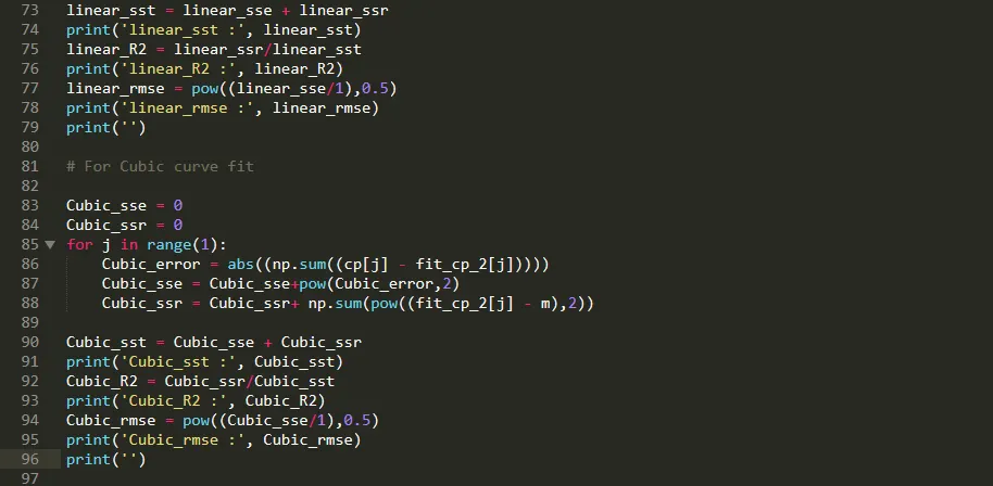
print('') - For characteristics of cubic fit:
Cubic_sse = 0
Cubic_ssr = 0
for j in range(1):
Cubic_error = abs((np.sum((cp[j] - fit_cp_2[j]))))
Cubic_sse = Cubic_sse+pow(Cubic_error,2)
Cubic_ssr = Cubic_ssr+ np.sum(pow((fit_cp_2[j] - m),2))Cubic_sst = Cubic_sse + Cubic_ssr
print('Cubic_sst :', Cubic_sst)
Cubic_R2 = Cubic_ssr/Cubic_sst
print('Cubic_R2 :', Cubic_R2)
Cubic_rmse = pow((Cubic_sse/1),0.5)
print('Cubic_rmse :', Cubic_rmse)
print('') - And printing their value of each.
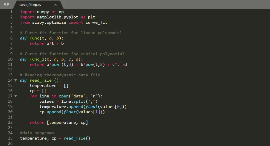
import numpy as np
import matplotlib.pyplot as plt
from scipy.optimize import curve_fit

# Curve_fit function for linear polynomial
def func(t, a, b):
	return a*t + b

# Curve_fit function for cubical polynomial
def func_1(t, a, b, c, d):
	return a*pow (t,3) + b*pow(t,2) + c*t +d

# Reading thermodynamic data file
def read_file ():
	temperature = []
	cp = []
	for line in open('data', 'r'):
		values = line.split(',')
		temperature.append(float(values[0]))
		cp.append(float(values[1]))

	return [temperature, cp]

#Main programs
temperature, cp = read_file()

popt, pcov = curve_fit(func, temperature, cp)
fit_cp_1 = func(np.array(temperature), *popt)
plt.plot(temperature, cp,, linewidth= 4)
plt.plot(temperature, fit_cp_1,, linewidth= 4)
plt.legend(['Actaual data', 'Curve_fit'])
plt.xlabel('temperature [k]')
plt.ylabel('cp')
plt.title('Linear Curve Fitting')
plt.show()

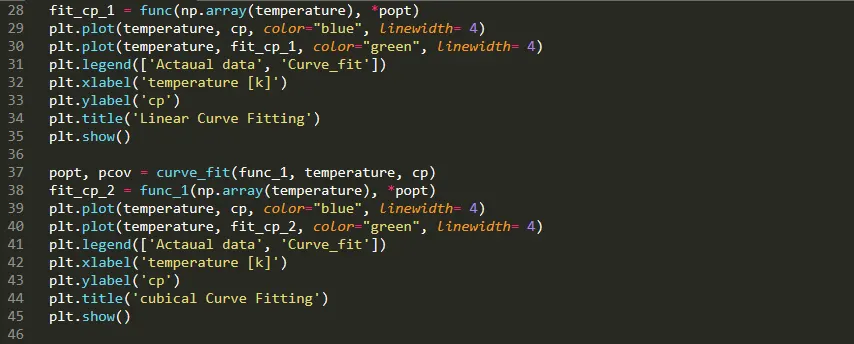
popt, pcov = curve_fit(func_1, temperature, cp)
fit_cp_2 = func_1(np.array(temperature), *popt)
plt.plot(temperature, cp,, linewidth= 4)
plt.plot(temperature, fit_cp_2,, linewidth= 4)
plt.legend(['Actaual data', 'Curve_fit'])
plt.xlabel('temperature [k]')
plt.ylabel('cp')
plt.title('cubical Curve Fitting')
plt.show()

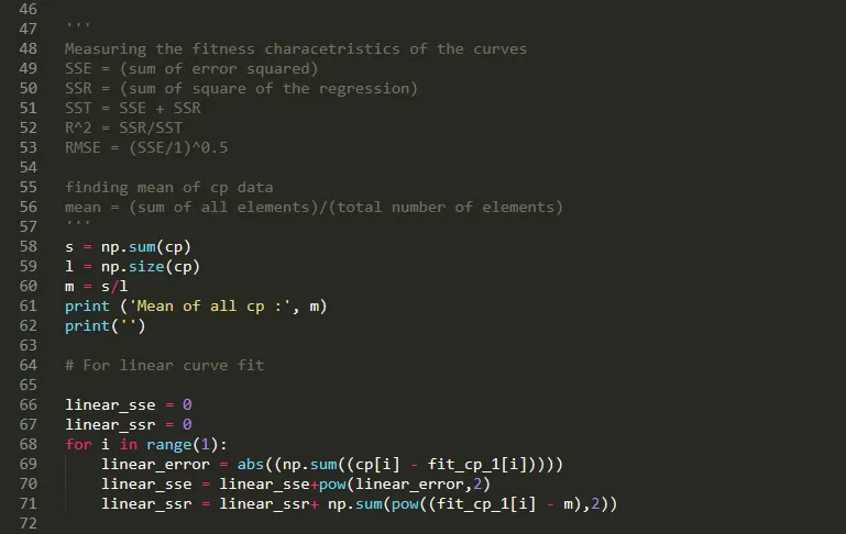
'''
Measuring the fitness characetristics of the curves
SSE = (sum of error squared)
SSR = (sum of square of the regression)
SST = SSE + SSR
R^2 = SSR/SST
RMSE = (SSE/1)^0.5

finding mean of cp data
mean = (sum of all elements)/(total number of elements)
'''
s = np.sum(cp)
l = np.size(cp)
m = s/l
print ('Mean of all cp :', m)
print('')

# For a linear curve fit

linear_sse = 0
linear_ssr = 0
for i in range(1):
	linear_error = abs((np.sum((cp[i] - fit_cp_1[i]))))
	linear_sse = linear_sse+pow(linear_error,2)
	linear_ssr = linear_ssr+ np.sum(pow((fit_cp_1[i] - m),2))

linear_sst = linear_sse + linear_ssr
print('linear_sst :', linear_sst)
linear_R2 = linear_ssr/linear_sst
print('linear_R2 :', linear_R2)
linear_rmse = pow((linear_sse/1),0.5)
print('linear_rmse :', linear_rmse)
print('')

# For Cubic curve fit

Cubic_sse = 0
Cubic_ssr = 0
for j in range(1):
	Cubic_error = abs((np.sum((cp[j] - fit_cp_2[j]))))
	Cubic_sse = Cubic_sse+pow(Cubic_error,2)
	Cubic_ssr = Cubic_ssr+ np.sum(pow((fit_cp_2[j] - m),2))

Cubic_sst = Cubic_sse + Cubic_ssr
print('Cubic_sst :', Cubic_sst)
Cubic_R2 = Cubic_ssr/Cubic_sst
print('Cubic_R2 :', Cubic_R2)
Cubic_rmse = pow((Cubic_sse/1),0.5)
print('Cubic_rmse :', Cubic_rmse)
print('')
RESULT
The graph of the linear curve fitting as plotted by the following code written:
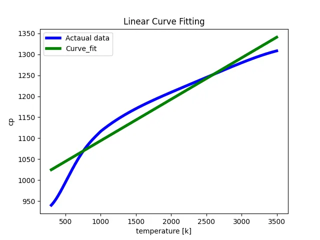
Fig 3: Linear curve fitting
The above graph shows the result for the linear curve vs actual data file between temperature and cp.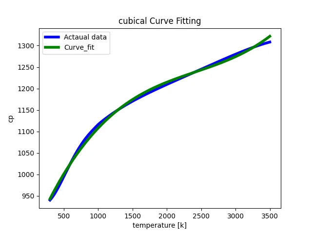
Fig 4: Cubical curve fitting
The above graph shows the result for the cubic curve vs actual data file between temperature and cp. The cubic curve is obtained is perfect for the actual data.
And the fit curve characteristics results obtained:
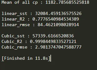
Hence it states that bend fit great R^2 ought to be near 1. It very well may be found from the outcomes got concerning straight bend fit R^2 is around 0.93 and for cubic bend fit it is about 0.99. so it tends to be said that cubic polynomial fits superior to straight polynomial. In the event that the request for the polynomial expands, the estimation of R^2 will creep towards 1 and fit will be thought to be acceptable.
APPENDIX
1) What do popt and pcov mean?
Ans. popt represents a matrix that stores and extracts the coefficients for the fitting functions according to general equations defined.
popt: array, optimal values for the parameters so that the sum of square residuals f(xdata, *popt) - ydata is minimized.
'pcov' represents the square matrix which stores the estimated values of covariance of the coefficients of the above. The diagonal elements of this square matrix also represent the variance of that coefficient.
pcov 2nd array
estimated covariance of popt, diagonals provide the variance of the parameter estimate, to compute one standard deviation errors on the parameters use perr = np.sqrt(np.diag(pcov)). How the sigma parameter affects the estimated covariance depends on the absolute_sigma argument. If true, as sigma used as absolute sense and the estimated parameter covariance pcov reflects these absolute values. If false, only the relative magnitudes of the sigma values matter
2) What does np.array (temperature) do?
Ans. This command converts each value of temperature in the data file into an array using the numpy module.
3) What does the *in*popt mean?
Ans. * in*popt indicates that the return of each coefficient stored in popt array.
4) What needs to be done in order to make the curve fit perfectly?
Ans. If we increase the order of the polynomial, the error produced will be less, and the curve fits perfectly. On increasing the order of the polynomial the value of R^2 will be close to 1 and assumed to perfect fit. The technique requires characterizing the capacities of each an ideal opportunity for another polynomial and can be viewed as long. Rather than this technique one of the information state temperatures can be part of numerous state temperature segments has 5000 information, we can part into 10 spaces of 500 qualities and the on-off chance that we plot them.
-----------------------------------------------------------------------------------------------------------------------------------------------------------------------------------------------------------------
Link: https://drive.google.com/drive/folders/1G6VA3LyObAsELmxKltIkE8O3FUUetIAD?usp=sharing