Week 5.1 - Mid term project - Solving the steady and unsteady 2D heat conduction problem

Question :

Steady state analysis & Transient State Analysis

Solve the 2D heat conduction equation by using the point iterative techniques that were taught in the class. The Boundary conditions for the problem are as follows;

Top Boundary = 600 K

Bottom Boundary = 900 K

Left Boundary = 400 K

Right Boundary = 800 K

You will implement the following methods for solving implicit equations.

• Jacobi
• Gauss-seidel
• Successive over-relaxation

Your absolute error criteria is 1e-4

2. You will write code for both implicit and explicit schemes (This is for the transient analysis only)

3. Compare the convergence rate [Number of iterations] of the steady state and transient [explicit and implicit] simulations and justify the numerics.

Answer

Heat conduction

Heat conduction is a fundamental process of heat transfer that occurs in solids, liquids, and gases. It refers to the transfer of thermal energy from a region of higher temperature to a region of lower temperature within a material or between different materials in direct physical contact, without any macroscopic motion of the material itself. This transfer of heat occurs due to the random motion of particles (atoms or molecules) within the material.

Example : A metal spoon left in a hot cup of coffee becomes warm due to heat conduction from the hot liquid to the spoon.

• 3-D transist heat conduction

`(dT)/(dt)+ alpha((d^2T)/(dx^2)+(d^2T)/(dy^2)+(d^2T)/(dz^2)) =0`

• 3-D steady state heat conduction

`(d^2T)/(dx^2)+(d^2T)/(dy^2)+(d^2T)/(dz^2) =0`

Differential equation

a differential equation expresses a relationship between a function and its derivatives, capturing how the function's behavior changes over the domain of the independent variable.

Types :

• Ordinary Differential Equations (ODEs):
• Partial Differential Equations (PDEs)

Methods to solve diffrential equation :

Direct numerical methods:

1. Euler's Method
2. Euler's Method
3. Adaptive Step Methods:
4. Finite Difference Methods
5. Finite Element Methods:
6. Boundary Element Methods
7. Spectral Methods:
8. Collocation Methods
9. Shooting Method
10. Implicit Methods

Iterative method

1. Fixed-Point Iteration
2. Newton's Method
3. Bisection Method
4. Jacobi Method:
5. Gauss-Seidel Method
6. Successive Over-Relaxation (SOR)

We are using 3 itrative solver method

For jacobbi

An iterative technique for solving systems of linear equations by updating each component of the solution vector based on the other components from the previous iteration.

For gauss

Similar to the Jacobi method, but it updates the components of the solution vector as soon as new values are available within each iteration.

For sor

An extension of the Gauss-Seidel method that introduces a relaxation parameter to potentially accelerate convergence.

According to question we are using 2-D heat conduction

• 2-D transist heat conduction

`(dT)/(dt)+ alpha((d^2T)/(dx^2)+(d^2T)/(dy^2)) = 0`

• 2-D steady state heat conduction

`(d^2T)/(dx^2)+(d^2T)/(dy^2) =0`

Discritization : Temprature is not the direction type . It flow in all direction so thats why we are using center discritization

1. 3-D steady state heat conduction

2. `(d^2T)/(dx^2)+(d^2T)/(dy^2)+(d^2T)/(dz^2) =0`

3. Implicit
6. `(T^(n+1)(i,j)-T^n(i,j))/(Deltat) +alpha((T(i+1,j)-2T(i,j)+T(i-1,j))/(Deltax^2)+(T(i,j+1)-2T(i,j)+T(i,j-1))/(Deltay^2))^(n+1)`

Step 2

`T^(n+1)(i,j)=T^n(i,j)+ +(Deltat)alpha((T(i+1,j)-2T(i,j)+T(i-1,j))/(Deltax^2)+(T(i,j+1)-2T(i,j)+T(i,j-1))/(Deltay^2))^(n+1)`

Step3

By solving above equation we get

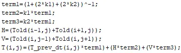
`T_(i,j) = (T_(prev)dt_(i,j))*(tearm_1) +H(tearm_2)+v(tearm_3)`

Where,

`K_1 = (alphaDeltat)/(Deltax^2)`

`K_2 = (alphaDeltat)/(Deltay^2)`

for jacobbi

for gauss

For sor

1. Explicit
2. `(T^(n+1)(i,j)-T^n(i,j))/(Deltat) = alpha((T(i+1,j)-2T(i,j)+T(i-1,j))/(Deltax^2)+(T(i,j+1)-2T(i,j)+T(i,j-1))/(Deltay^2))^n`

Step 1

`T^(n+1)(i,j)=T^n(i,j)+K_1(T(i+1,j)-2T(i,j)+T(i-1,j))+K_2(T(i,j+1)-2T(i,j)+T(i,j-1))`

Where,

`K_1 = (alphaDeltat)/(Deltax^2)`

`K_2 = (alphaDeltat)/(Deltay^2)`

Steady State :

`(delta^2T)/(deltax^2) + (delta^2T)/(deltay^2) = 0`

`(T(i+1,j)-2T(i,j)+T(i-1,j))/(Deltax^2)+(T(i,j+1)-2T(i,j)+T(i,j-1))/(Deltay^2) = 0`

`2T_(i,j)/(Deltax^2) + 2T_(i,j)/(Deltay^2) = (T_(i+1,j) +T_(i-1,j))/(Deltax^2) +(T(i,j+1)+T(i,j-1))/(Deltay^2)`

`T_(i,j) = ((T_(i+1,j) +T_(i-1,j))/(Deltax^2) +(T(i,j+1)+T(i,j-1))/(Deltay^2))/k`

where

`k =(2(Deltax^2 + Deltay^2))/(Deltax^2Deltay^2`

for jacobbi

for gauss

For sor

Steady state

Explanation :

CODE :

%initial conditions
%L = 1
nx = 10;
ny = 10;
x = linspace(0,1,nx);
y = linspace(0,1,ny);
dx = x(2) - x(1);
dy = y(2) - y(1);


% given data of boundary condition
% initial temp condition

t = 300*ones(nx,ny);  
t(:,1) = 400;
t(1,:) = 600;
t(:,ny) = 800;
t(nx,:) = 900;

% defining the temperature at corner points

t(1,1) = 500;
t(nx,ny) = 850;
t(1,ny) = 700;
t(nx,1) = 650;

dt = 1e-2; %time step
told=t;

error = 100;
tol = 1e-4;
k = 2*(dx^2+dy^2)/(dx^2*dy^2);
% k2 = (dy^2)/(2*(dx^2+dy^2));

method = input('Iterative method = '); %iterative method selection

%JACOBI ITERATIVE METHOD

if (method==1)
    tic;
    jacobi = 1;
    while(error>tol)
        for i = 2:(nx-1)
            for j = 2:(ny-1)
            t(i,j) = (((told(i-1,j)+told(i+1,j))/(dx^2))+((told(i,j+1)+told(i,j-1))/(dy^2)))/k;
            end
        end
    error = max(max(abs(t-told)));
    told = t;
    jacobi = jacobi+1;
    time_taken = toc;
    end

%plotting    
figure(1)
contourf(x,y,t,'ShowText','on');
colormap(jet);
colorbar;
xlabel('X')
ylabel('Y')
text1 = sprintf('number of iteration = %d', jacobi);
text2 = sprintf('simulation time = %f', time_taken);
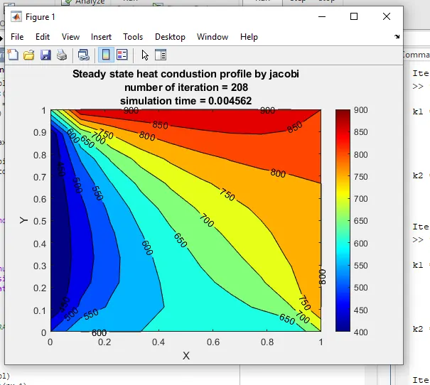
title({'Steady state heat condustion profile by jacobi'; text1; text2});
end


%GAUSS-SEIDEL ITERATIVE METHOD

if (method==2)
    tic;
    gauss = 1;
    while(error>tol)
        for i = 2:(nx-1)
            for j = 2:(ny-1)
            t(i,j) = (((t(i-1,j)+told(i+1,j))/(dx^2))+((told(i,j+1)+t(i,j-1))/(dy^2)))/k;
            end
        end
    error = max(max(abs(t-told)));
    told = t;
    gauss = gauss+1;
    time_taken = toc;
    end

%plotting
figure(2)
contourf(x,y,t,'ShowText','on');
colormap(jet);
colorbar;
xlabel('X')
ylabel('Y')
text1 = sprintf('number of iteration = %d', gauss);
text2 = sprintf('simulation time = %f', time_taken);
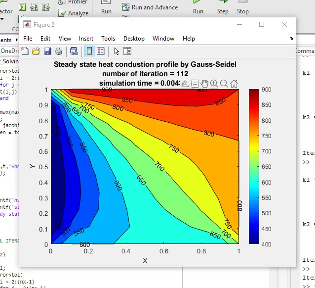
title({'Steady state heat condustion profile by Gauss-Seidel'; text1; text2});
end


%SUCCESSIVE OVER RELAXATION ITERATIVE METHOD

if (method==3)
    tic;
    sor = 1;
    omega = 1.4; %over relaxation factor
    while(error>tol)
        for i = 2:(nx-1)
            for j = 2:(ny-1)
            term1 =(t(i-1,j)+told(i+1,j))/(dx^2);
            term2 =(told(i,j+1)+t(i,j-1))/(dy^2);
            t(i,j) = ((told(i,j)*(1-omega)))+(omega*(term1+term2))/k;
            end
        end
    error = max(max(abs(t-told)));
    told = t;
    sor = sor+1;
    time_taken = toc;
    end

%plotting
figure(3)
contourf(x,y,t,'ShowText','on');
colormap(jet);
colorbar;
xlabel('X')
ylabel('Y')
text1 = sprintf('number of iteration = %d', sor);
text2 = sprintf('simulation time = %f', time_taken);
text3 = sprintf('over relaxation factor = %f', omega);
title({'Steady state heat condustion profile by Successive Over Relaxation'; text1; text2; text3});
end

Resut :

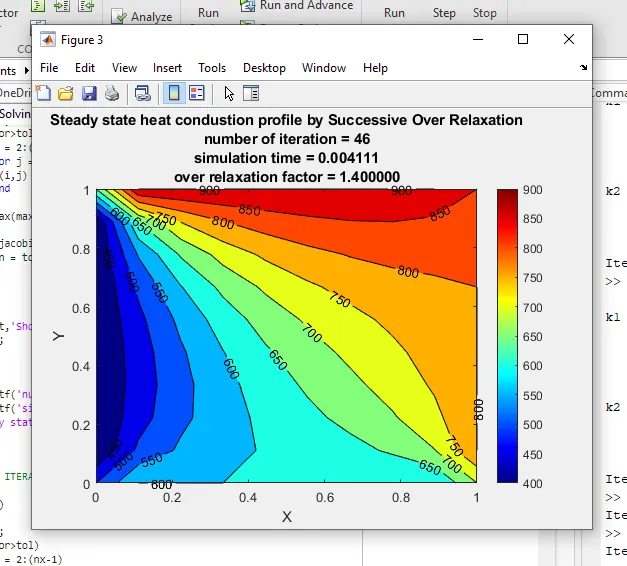
Transist State Implicit

Explaination :

1. Initial Setup:

   • The code sets up the initial conditions for the simulation. The domain is a 2D square with dimensions nx by ny. The number of time steps is given by nt.
   • It creates a grid of spatial coordinates x and y using linspace, and calculates the grid spacing dx and dy.
   • The initial temperature distribution t is set to 300 everywhere in the domain.
   • Specific boundary temperatures are defined for the four sides of the domain, and corner temperatures are also set.

2. Time Step and Thermal Diffusivity:

   • The time step dt is set for the transient simulation. This parameter determines the time interval between each time step.
   • The thermal diffusivity alpha is defined, which relates to how quickly heat is conducted through the material.

3. Iterative Methods:

   • The user is prompted to input the desired iterative method(jacobi,gauss,sor) to solve the transient heat conduction equation.

4. Jacobi Iterative Method:

   • If the selected method is Jacobi (method 1), the code proceeds with this section.
   • For each time step (p), it enters a loop to iteratively update the temperature distribution t until a convergence criterion is met (controlled by the error and tol variables).
   • Nested loops iterate over the interior points of the domain (excluding boundaries) and update the temperature at each point using a discretized form of the heat equation.
   • The told matrix stores the previous temperature distribution, and tprev_dt is used to track the previous time step's temperature.
   • The error between the current and previous temperature distributions is calculated and checked against the tolerance tol.
   • The number of iterations (jacobi) is counted, and the updated told matrix is stored.
   • After completing the iterative process for all time steps, the temperature distribution is plotted using a contour plot.

5. Gauss-Seidel Iterative Method:

   • Similar to the Jacobi method, but the Gauss-Seidel approach updates temperature values using the most recently calculated values within the same iteration. This can lead to faster convergence.
   • The temperature update loops are nested within time step loops, and the same convergence criteria are used.

6. Successive Over Relaxation (SOR) Iterative Method:

   • This section applies the Successive Over Relaxation method to solve the transient heat conduction equation.
   • The SOR method enhances convergence by applying an over relaxation factor omega.
   • Temperature update loops are nested within time step loops, similar to the other methods.

7. Plotting:

   • After completing the iterative process for all time steps and selected method, the temperature distribution at the final time step is plotted using a contour plot.
   • The colormap jetis applied for visualization, and color bars indicate temperature values.
   • Labels and titles are added to the plot to provide information about the simulation.

CODE :

%initial conditions
%L = 1
nx = 10;
ny = 10;
nt = 300; % No.of steps
x = linspace(0,1,nx);
y = linspace(0,1,ny);
dx = x(2) - x(1);
dy = y(2) - y(1);


% given data of boundary condition
% initial temp condition

t = 300*ones(nx,ny);  
t(:,1) = 400;
t(1,:) = 600;
t(:,ny) = 800;
t(nx,:) = 900;

% defining the temperature at corner points

t(1,1) = 500;
t(nx,ny) = 850;
t(1,ny) = 700;
t(nx,1) = 650;

dt = 0.01; %time step
told=t;
alpha = 0.3; % Thermal diffusivity
tprev_dt = told;

tol = 1e-4;
k1 = alpha*dt/(dx^2);
k2 = alpha*dt/(dy^2);

method = input('Iterative method = '); %iterative method selection

%JACOBI ITERATIVE METHOD

if (method==1)
    tic;
    jacobi = 1;
    for p = 1:nt
        error =100;
         while(error>tol)
        for i = 2:(nx-1)
            for j = 2:(ny-1)
                term1 = (1+(2*k1)+(2*k2))^-1;
                term2 = k1*term1;
                term3 = k2*term1;
                h = (told(i-1,j)+told(i+1,j));
                v = (told(i,j+1)+told(i,j-1));
                t(i,j) = ((tprev_dt(i,j)*term1)+(h*term2)+(v*term3));
            end
        end
        
    error = max(max(abs(t-told)));
    told = t;
    jacobi = jacobi+1;
         end
         tprev_dt = t ;
    end
    time_taken = toc;

%plotting    
figure(1)
contourf(x,y,t,'ShowText','on');
colormap(jet);
colorbar;
xlabel('X')
ylabel('Y')
text1 = sprintf('number of iteration = %d', jacobi);
text2 = sprintf('simulation time = %f', time_taken);
title({'Transient state heat conduction profile Implicit-Jacobi'; text1; text2});
end


%GAUSS-SEIDEL ITERATIVE METHOD

if (method==2)
    tic;
    gauss = 1;
    for p = 1:nt
        error =100;
         while(error>tol)
        for i = 2:(nx-1)
            for j = 2:(ny-1)
                term1 = (1+(2*k1)+(2*k2))^-1;
                term2 = k1*term1;
                term3 = k2*term1;
                h = (t(i-1,j)+told(i+1,j));
                v = (told(i,j+1)+t(i,j-1));
                t(i,j) = ((tprev_dt(i,j)*term1)+(h*term2)+(v*term3));
            end
        end
        
    error = max(max(abs(t-told)));
    told = t;
    gauss = gauss+1;
         end
         tprev_dt = t; 
    end
    time_taken = toc;

%plotting    
figure(1)
contourf(x,y,t,'ShowText','on');
colormap(jet);
colorbar;
xlabel('X')
ylabel('Y')
text1 = sprintf('number of iteration = %d', gauss);
text2 = sprintf('simulation time = %f', time_taken);
title({'Transient state heat conduction profile Implicit-Gauss-seidel'; text1; text2});
end

%SUCCESSIVE OVER RELAXATION ITERATIVE METHOD

if (method==3)
    tic;
    sor = 1;
    omega = 1.2; % Over relaxation factor
    for p = 1:nt
        error =100;
         while(error>tol)
        for i = 2:(nx-1)
            for j = 2:(ny-1)
                term1 = (1+(2*k1)+(2*k2))^-1;
                term2 = k1*term1;
                term3 = k2*term1;
                h = (t(i-1,j)+told(i+1,j));
                v = (told(i,j+1)+t(i,j-1));
                t(i,j) = (told(i,j)*(1-omega))+(omega*((tprev_dt(i,j)*term1)+(h*term2)+(v*term3)));
            end
        end
        
    error = max(max(abs(t-told)));
    told = t;
    sor = sor+1;
         end
         tprev_dt = t ;
    end
    time_taken = toc;

%plotting    
figure(1)
contourf(x,y,t,'ShowText','on');
colormap(jet);
colorbar;
xlabel('X')
ylabel('Y')
text1 = sprintf('number of iteration = %d', sor);
text2 = sprintf('simulation time = %f', time_taken);
title({'Transient state heat conduction profile Implicit-SOR'; text1; text2});
end

Result :

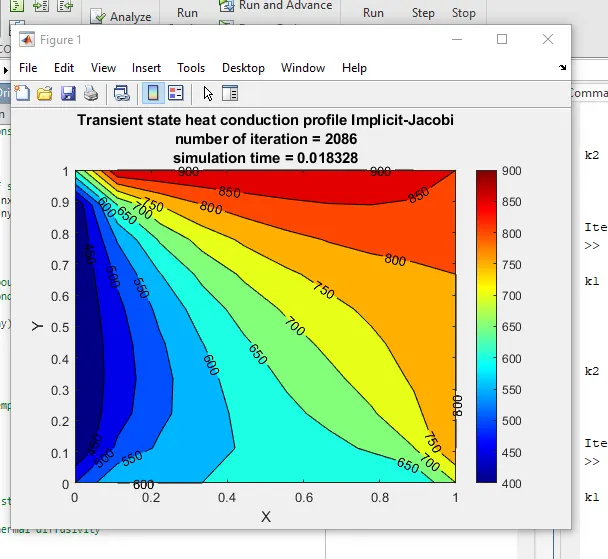
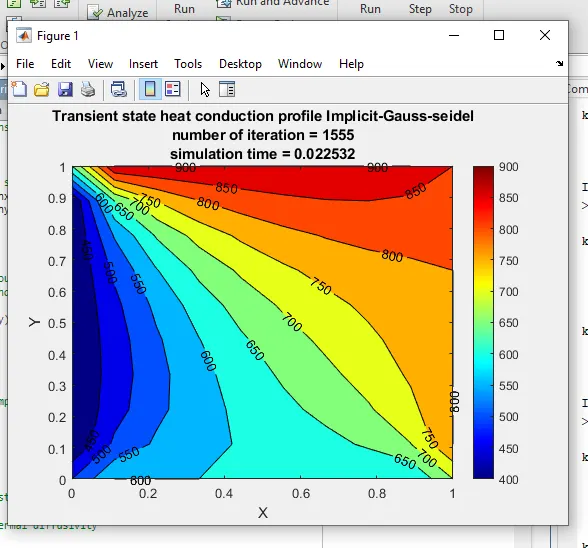
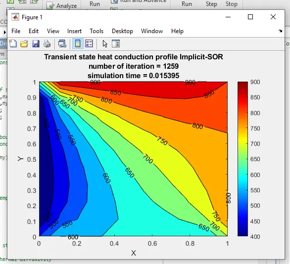
Transist State -Explicit

Code:

%initial conditions
%L = 1
nx = 10;
ny = 10;
x = linspace(0,1,nx);
y = linspace(0,1,ny);
dx = x(2) - x(1);
dy = y(2) - y(1);


% given data of boundary condition
% initial temp condition

t = 300*ones(nx,ny);  
t(:,1) = 400;
t(1,:) = 600;
t(:,ny) = 800;
t(nx,:) = 900;

% defining the temperature at corner points

t(1,1) = 500;
t(nx,ny) = 850;
t(1,ny) = 700;
t(nx,1) = 650;

dt = 1e-2; %time step
tprev=t;
alpha = 0.1;
error = 100;
tol = 1e-4;
k1 = (alpha*dt)/(dx)^2;
k2 = (alpha*dt)/(dy)^2;



    tic;
    iter = 1;
    while(error>tol)
        for i = 2:(nx-1)
            for j = 2:(ny-1)
                t(i,j)=tprev(i,j)+k1*(tprev(i+1,j)-2*tprev(i,j)+tprev(i-1,j))+k2*(tprev(i,j+1)-2*tprev(i,j)+tprev(i,j-1));
            end
        end
    error = max(max(abs(t-tprev)));
    tprev = t;
    iter = iter+1;
    time_taken = toc;
     end
CFL = (alpha*dt)/(dx^2) + (alpha*dt)/(dy^2);

%plotting
figure(3)
contourf(x,y,t,'ShowText','on');
colormap(jet);
colorbar;
xlabel('X')
ylabel('Y')
text1 = sprintf('number of iteration = %d', iter);
text2 = sprintf('simulation time = %f', time_taken);
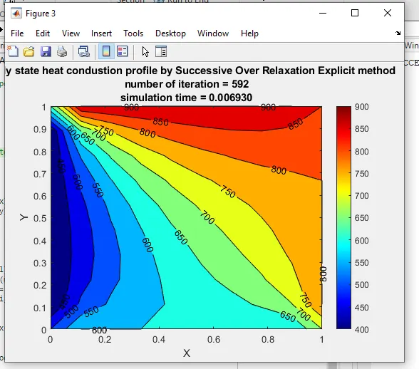
title({'Steady state heat condustion profile by Successive Over Relaxation Explicit method'; text1; text2});
   

Explaination :

1. Initialization:

   • nx and ny are set to define the number of grid points in the x and y directions.
   • x and y are created using linspace, which generates evenly spaced coordinates within the range [0, 1] along the x and y directions.
   • dx and dyare calculated as the differences between adjacent grid points along the x and y directions.

2. Initial Temperature and Boundary Conditions:

   • A matrix t of size nx by ny is created to represent the temperature distribution in the domain.
   • The initial temperature is set to 300K for all grid points.
   • Specific boundary conditions are applied: the left boundary (t(:,1)), top boundary (t(1,:)), right boundary (t(:,ny)), and bottom boundary (t(nx,:)) are set to fixed temperatures.
   • The corner points' temperatures are also explicitly defined.

3. Time Step and Parameters:

   • dt is set as the time step for the simulation.
   • tprev is initialized to store the previous temperature distribution for iterative updates.
   • alpha is a coefficient related to thermal diffusivity.
   • error is initialized to a high value to start the iterative process.
   • tol is the tolerance that determines when the iteration will stop.
   • k1 and k2 are coefficients used in the finite-difference equations to update temperatures.

4. Main Iterative Loop:

   • The code enters a while loop that continues as long as the error is greater than the specified tolerance tol.
   • Two nested loops iterate over the interior grid points, excluding the boundaries.
   • The new temperature at each grid point is calculated using the explicit finite-difference method for heat conduction. The change in temperature is based on neighboring points and time step, considering both the x and y directions.

5. Convergence Check and Updating:

   • After each iteration of the nested loops, the maximum change in temperature (error) is calculated across all grid points using the max function and the absolute difference between t and tprev.
   • If the error is less than tol, the simulation is considered to have converged, and the iteration will stop. Otherwise, the iteration continues.

6. Updating tprev and Iteration Count:

   • The tprev matrix is updated with the newly calculated temperature distribution t for the next iteration.
   • The iteration count iter is incremented by one.

7. Plotting:

   • Once the simulation has converged, a contour plot of the temperature distribution is created using contourf, which generates a filled contour plot.
   • The colormap, colorbar, labels, and title are set to make the plot informative.
   • The number of iterations and the simulation time are added to the title for context.

8. CFL Calculation:

   • The Courant-Friedrichs-Lewy (CFL) condition, which relates time step and grid spacing to stability in numerical simulations, is calculated and stored in CFL.

Result