Week 5.1 - Mid term project - Solving the steady and unsteady 2D heat conduction problem
The heat equation is a second order partial differential equation that describes how the distribution of some quantity such as heat evolves over time in a solid medium, as it spontaneously flows from place where it is higher towards places where it is lower. It is a special case of the diffusion equation.
For a function
Where, alpha (
In compact form,
his equation describes the flow of heat in homogeneous and isotropic medium, with
Informally, the laplacian operator
The above equation is solved on a 2-D plate which contains four boundaries and the value at those boundaries are:
The value of thermal diffusivity is taken as 1.4, because more value will give the solution faster.
The assumption made to solve above equation on a 2-D plate are:
- The material is homogeneous and isotropic
- The Alpha is not the function of temperature.
- The radiative and convective losses are neglected.
The final solution is obtained in three ways
- Neglecting unsteady term in the equation (steady state solution).
- Considering unsteady term but solved by explicit method.
- Considering unsteady term but solved by implicit method.
The numerical method used to solve the heat equation for all the above cases is finite difference method. The second order accurate FDM for space term and first order accurate FDM for time term is used to get the solution. So general 2D FDM form of the equation will be;
The above form will be modified according to the above three cases and the solution will be obtained.
CODE EXPLANATION for Unsteady State
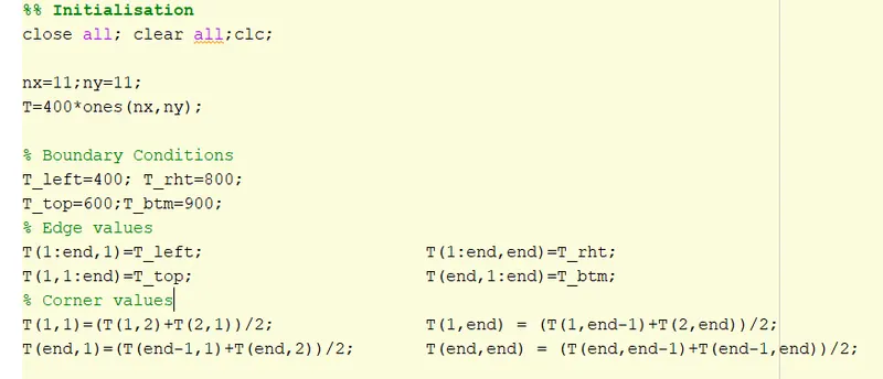
Giving number of nodes as nx and ny, nx=ny=11;
Assign boundary conditions as given in question. After that assign corner values as the mean of 2 edge values
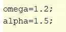
Then initialise the values of omega and alpha to be used in equation
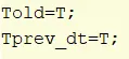
Put the Temperature values in other 2 variables so as to use it as old values in forward space method and time marching method.
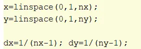
Put the computational domain in terms of x and y and divide it into equal intervals with dx and dy values.
Use the keyword input to obtain time step values, Implicit/Explicit method and step size

Then calculate the values of kx and ky to be used in equation

If we use implicit method, we have 3 iterative solvers which are Jacobi, Guass Siedel and Sor method. Choose any 3.
The iteration procedure may vary in 3 cases
After giving time marching loop, initialise the value for error and tolerance such that after every the equation needs to be iterated so as to get the converged value.
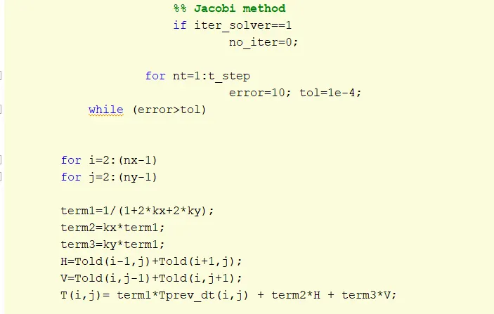
a) Jacobi method
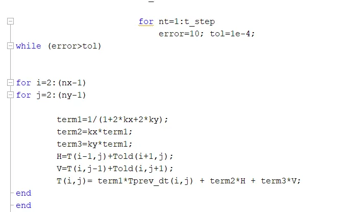
b) Guass Siedel method
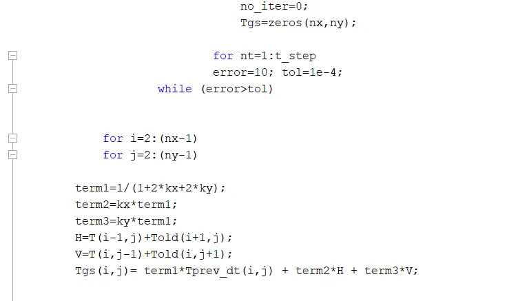
c) SOR method
After iterating the space loop, find the value of maximum error getting. error = Told - T;
After that, initialise the value of Told as T.
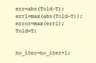
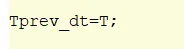
Then end that convergence loop. Then initialise Tprev_dt=T; so as to update the new time step value in previous time step and to use it as previous time step in next time marching.
Then go for plotting the solution
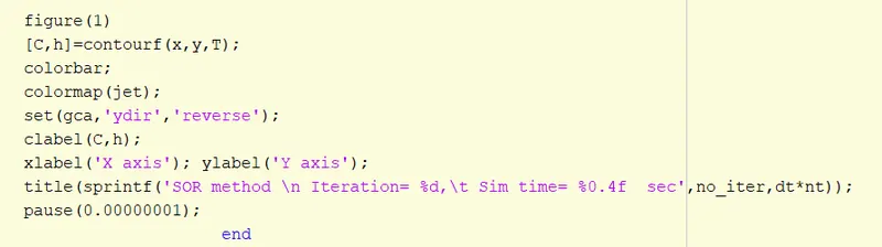
Then end the time loop and see how the value changes after every time step. If we don't want to see the values changing after every time step, we can plot it outside the time loop.
Now go for explicit method
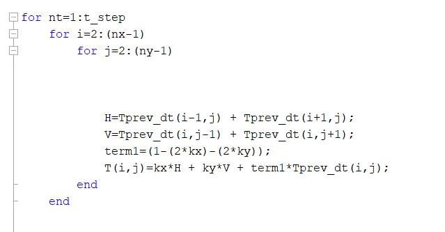
In explicit method, we are not iterating because all the known values are at same time step.
The equation write in matlab are based on formulas given in tutorial videos
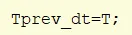
Then initialise Tprev_dt=T; so as to update the new time step value in previous time step and to use it as previous time step in next time marching.
After that go for plotting the solution
CODE EXPLANATION for Steady State
In steady state,
So,
The kx and ky values are changed from unsteady state. It is shown below

All the other methods are same as unsteady state. Here, we don't use the time loop.
Case I. Solution by neglecting unsteady term(STEADY STATE).
The FDM form for the steady state equation will be:
The equation will be solved using Jacobi, Gauss seidel, Successive over relaxation iteration method to check that which method is faster and how it works.
MATLAB code
close all; clear all;clc;

T_left=400; T_rht=800;
T_top=600;T_btm=900;

tol=1e-4;

nx=11;ny=11;
T=300*ones(nx,ny);

T(1:end,1)=T_left;                      T(1:end,end)=T_rht;
T(1,2:end-1)=T_top;                     T(end,2:end-1)=T_btm;
T(1,1)=(T(1,2)+T(2,1))/2;               T(1,end) = (T(1,end-1)+T(2,end))/2;
T(end,1)=(T(end-1,1)+T(end,2))/2;       T(end,end) = (T(end,end-1)+T(end-1,end))/2;
omega=1.5;


Told=T;
Tprev_dt=T;
alpha=1.5;


x=linspace(0,1,nx);
y=linspace(0,1,ny);
dx=1/(nx-1); dy=1/(ny-1);

kxs=(dy^2)/(2*((dx^2)+(dy^2)));
kys=(dx^2)/(2*((dx^2)+(dy^2)));


error=10;

iter_solver = input('Enter 1 for jacobi or 2 for gauss siedel or 3 for sos = ');
                        %% Jacobi method
                        if iter_solver==1
                        no_iter=0;


while (error>tol)


for i=2:(nx-1)
for j=2:(ny-1)


        H=Told(i-1,j)+Told(i+1,j);
        V=Told(i,j-1)+Told(i,j+1);
        T(i,j)= kxs*H + kys*V;
end
end

        err=abs(Told-T)
        err1=max(abs(Told-T));
        error=max(err1);
        Told=T;


        no_iter=no_iter+1;

        figure(1)
        [C,h]=contourf(x,y,T)
        colorbar
        colormap(jet)
        clabel(C,h)
        title(sprintf('Jacobi= %d',no_iter));
        set(gca,'ydir','reverse')
        pause(0.03);


end


                        end


                        %% GS method
                        if iter_solver==2
                        no_iter=0;
while (error>tol)


for i=2:(nx-1)
for j=2:(ny-1)


        H=T(i-1,j)+Told(i+1,j);
        V=T(i,j-1)+Told(i,j+1);
        T(i,j)= kxs*H + kys*V;
end
end

        err=abs(Told-T)
        err1=max(abs(Told-T));
        error=max(err1);
        Told=T;


        no_iter=no_iter+1;

        figure(1)
       [C,h]=contourf(x,y,T)
       colorbar
       colormap(jet)
       clabel(C,h)
       title(sprintf('Gauss Siedel= %d',no_iter));
       set(gca,'ydir','reverse')
       pause(0.03);


end


                        end


                        %% Successive Over Relaxation method
                        if iter_solver==3
                        no_iter=0;
                        Tgs=zeros(nx,ny);
while (error>tol)


for i=2:(nx-1)
for j=2:(ny-1)


        H=T(i-1,j)+Told(i+1,j);
        V=T(i,j-1)+Told(i,j+1);
        Tgs(i,j)= kxs*H + kys*V;

        T(i,j)=(1-omega)*Told(i,j)+omega*Tgs(i,j);
end
end

        err=abs(Told-T)
        err1=max(abs(Told-T));
        error=max(err1);
        Told=T;


        no_iter=no_iter+1;

       figure(1)
       [C,h]=contourf(x,y,T)
       colorbar
       colormap(jet)
       clabel(C,h)
       title(sprintf('Successive Over Relaxation= %d',no_iter));
       set(gca,'ydir','reverse')
       pause(0.03);


end


                        end
As we are observing the steady temperature distribution in the plate, the final solution with all the method will be visually same, but the number of iterations of each method will be different.
The temperature distribution plot with the number of iterations are;
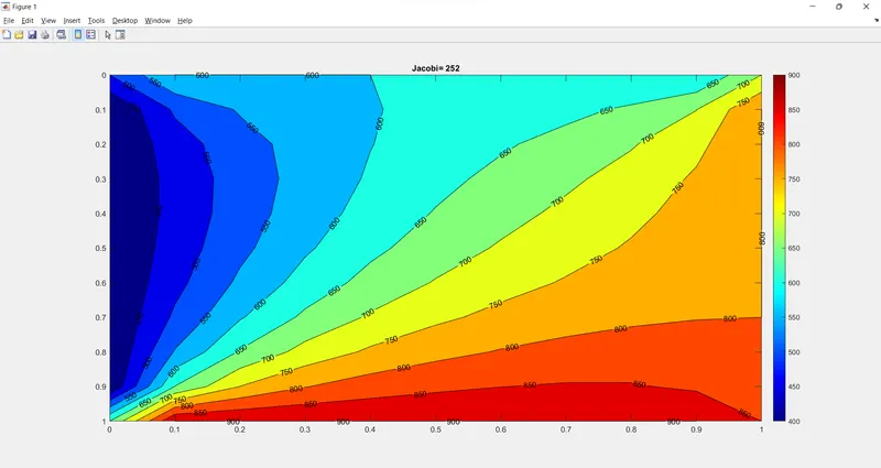
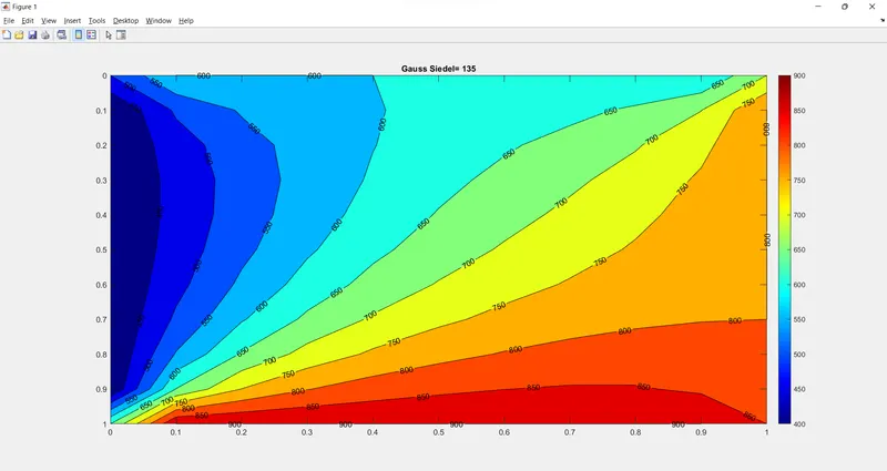
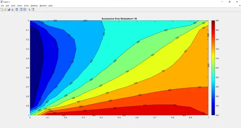
The above graph clearly shows that SOR method takes the smaller number of iterations to converge than the Gauss Seidel and Jacobi. Consequently, d SOR takes less time followed by Gauss Seidel and Jacobi method. To get the solution faster, the successive relaxation factor should be optimum. In above case the relaxation factor from 1-2 to has been tried and the factor 1.5 has given the solution in least number of iterations.
As per the error criteria given, the final solution will be the same, but the method to get the solution faster is also equally important. And, SOR is the winner.
Case II. Solution by considering unsteady term
a) explicit method
The explicit form of the above equation is easy to form but care should be taken to get the stable solution. The CFL condition based timestep is required to get the stable solution.
the finite difference explicit form of the equation is:
Solving we get
For stable criteria
As the solution for the previous time exist for time marching, this form of the solution is easy to solve. The iterative solvers are not required for this method because system of equations is not getting form. The RHS of the equation is completely known and there is only one unknown in the equation. so, the simple and sort code for this method is,
b) implicit method
The implicit method is unconditionally stable but it is difficult and time consuming. Application of implicit method on each node will form a system of linear equations and it needs to be solved by iterative methods. The iterative methods are discussed in the steady state solution and to maintain the consistency, same methods are used in this method.
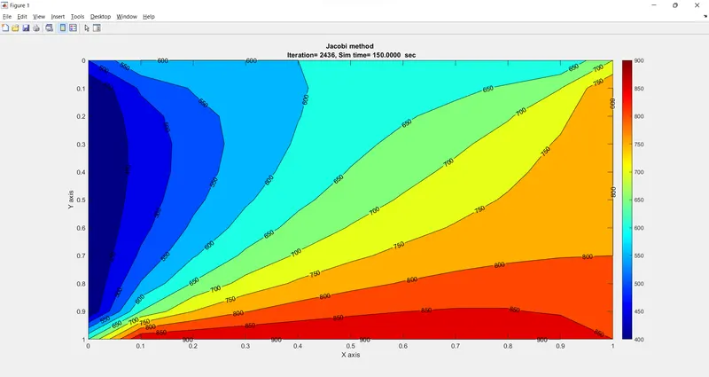
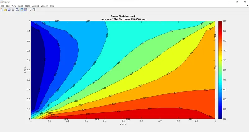
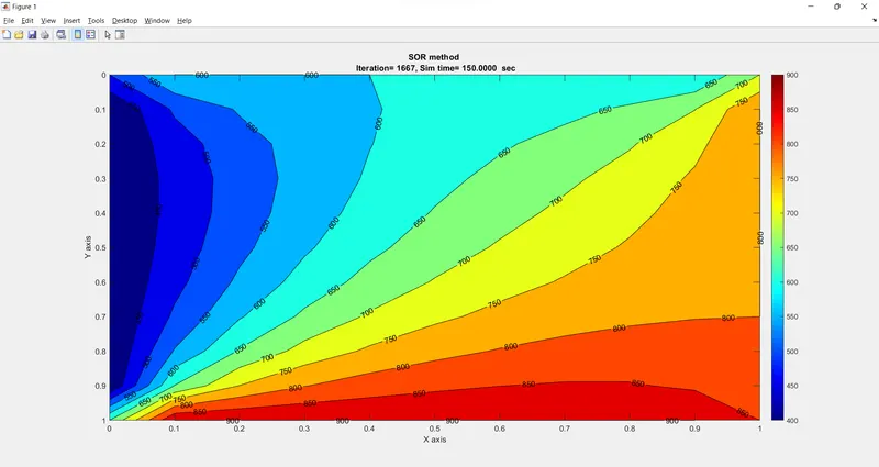
The results of 3 methods are also observed to be same as before, in which SOR will take least iterations followed by Gauss Seidel and Jacobi.
The CFL criteria is not required to be checked for calculating timestep. The total iterations and total number of time steps are calculated and compared for all the three methods.
MATLAB CODE for unsteady state
%% Initialisation
close all; clear all;clc;

nx=11;ny=11;
T=400*ones(nx,ny);

% Boundary Conditions
T_left=400; T_rht=800;
T_top=600;T_btm=900;
% Edge values
T(1:end,1)=T_left;                      T(1:end,end)=T_rht;
T(1,1:end)=T_top;                       T(end,1:end)=T_btm;
% Corner values
T(1,1)=(T(1,2)+T(2,1))/2;               T(1,end) = (T(1,end-1)+T(2,end))/2;
T(end,1)=(T(end-1,1)+T(end,2))/2;       T(end,end) = (T(end,end-1)+T(end-1,end))/2;


omega=1.5;
alpha=1.5;

Told=T;
Tprev_dt=T;

x=linspace(0,1,nx);
y=linspace(0,1,ny);

dx=1/(nx-1); dy=1/(ny-1);

error=10;  tol=1e-4;
err=zeros(nx,ny);

t_step =  input('Enter time step = ');
method =  input('Enter 1 for implicit or Enter 2 for explicit = ');
dt     =  input('Enter step size dt = ');

kx=alpha*dt/(dx^2);             ky=alpha*dt/(dy^2);

%% Implicit method

if method ==1
iter_solver = input('Enter 1 for jacobi or 2 for gauss siedel or 3 for sos = ');
                        %% Jacobi method
                        if iter_solver==1
                                no_iter=0;

                    for nt=1:t_step
                                error=10; tol=1e-4;
            while (error>tol)


        for i=2:(nx-1)
        for j=2:(ny-1)

        term1=1/(1+2*kx+2*ky);
        term2=kx*term1;
        term3=ky*term1;
        H=Told(i-1,j)+Told(i+1,j);
        V=Told(i,j-1)+Told(i,j+1);
        T(i,j)= term1*Tprev_dt(i,j) + term2*H + term3*V;


        end
        end

        err=abs(Told-T);
        err1=max(abs(Told-T));
        error=max(err1);
        Told=T;


        no_iter=no_iter+1;

               end
        Tprev_dt=T;

        figure(1)
        [C,h]=contourf(x,y,T);
        colorbar;
        colormap(jet);
        set(gca,'ydir','reverse');
        clabel(C,h);
        xlabel('X axis'); ylabel('Y axis');
        title(sprintf('Jacobi method \n Iteration= %d,\t Sim time= %0.4f  sec',no_iter,dt*nt));
        pause(0.00000001);
                    end
                        end


                        %% GS method
                        if iter_solver==2
                        no_iter=0;

                        for nt=1:t_step
                            error=10; tol=1e-4;
while (error>tol)


for i=2:(nx-1)
for j=2:(ny-1)

        term1=1/(1+2*kx+2*ky);
        term2=kx*term1;
        term3=ky*term1;
        H=T(i-1,j)+Told(i+1,j);
        V=T(i,j-1)+Told(i,j+1);
        T(i,j)= term1*Tprev_dt(i,j) + term2*H + term3*V;
end
end

        err=abs(Told-T);
        err1=max(abs(Told-T));
        error=max(err1);
        Told=T;


        no_iter=no_iter+1;


end
Tprev_dt=T;

        figure(1)
        [C,h]=contourf(x,y,T);
        colorbar;
        colormap(jet);
        set(gca,'ydir','reverse');
        clabel(C,h);
        xlabel('X axis'); ylabel('Y axis');
        title(sprintf('Gauss Siedel method \n Iteration= %d,\t Sim time= %0.4f  sec',no_iter,dt*nt));
        pause(0.00000001);
        end


                        end

                         %% Successive Over Relaxation method
                        if iter_solver==3
                                no_iter=0;
                                Tgs=zeros(nx,ny);

                            for nt=1:t_step
                            error=10; tol=1e-4;
                    while (error>tol)


            for i=2:(nx-1)
            for j=2:(ny-1)

        term1=1/(1+2*kx+2*ky);
        term2=kx*term1;
        term3=ky*term1;
        H=T(i-1,j)+Told(i+1,j);
        V=T(i,j-1)+Told(i,j+1);
        Tgs(i,j)= term1*Tprev_dt(i,j) + term2*H + term3*V;


        T(i,j)=(1-omega)*Told(i,j)+omega*Tgs(i,j);
            end
            end

        err=abs(Told-T);
        err1=max(abs(Told-T));
        error=max(err1);
        Told=T;


        no_iter=no_iter+1;

                    end
Tprev_dt=T;

        figure(1)
        [C,h]=contourf(x,y,T);
        colorbar;
        colormap(jet);
        set(gca,'ydir','reverse');
        clabel(C,h);
        xlabel('X axis'); ylabel('Y axis');
        title(sprintf('SOR method \n Iteration= %d,\t Sim time= %0.4f  sec',no_iter,dt*nt));
        pause(0.00000001);
                            end


                        end


end


%         figure(1)
%         [C,h]=contourf(x,y,T)
%         colorbar
%         colormap(jet)
%         set(gca,'ydir','reverse')
%         clabel(C,h);
%         xlabel('X axis'); ylabel('Y axis');
%         title(sprintf('Jacobi method \n Iteration= %d,\t Sim time= %0.4f  sec',no_iter,dt*nt));


%% Explicit method


if method==2

for nt=1:t_step
    for i=2:(nx-1)
        for j=2:(ny-1)


            H=Tprev_dt(i-1,j) + Tprev_dt(i+1,j);
            V=Tprev_dt(i,j-1) + Tprev_dt(i,j+1);
            term1=(1-(2*kx)-(2*ky));
            T(i,j)=kx*H + ky*V + term1*Tprev_dt(i,j);
        end
    end


        err=abs(Tprev_dt-T);
        err1=max(abs(Tprev_dt-T));
        error=max(err1);

        Tprev_dt=T;

        figure(1)
        [C,h]=contourf(x,y,T);
        colorbar;
        colormap(jet);
        set(gca,'ydir','reverse');
        clabel(C,h);
        xlabel('X axis'); ylabel('Y axis');
        title(sprintf('Explicit method \n Sim time= %0.4f  sec',dt*nt));
        pause(0.00000001);

end
end
Implicit output plot
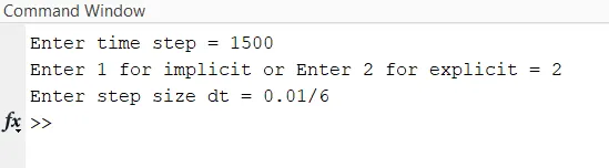
Enter time step = 1500; Enter 1 for implicit; Enter dt = 0.1 sec, Then Simulation time = 1500*0.1 = 150 sec
a) Jacobi
b) Gauss Siedel
c) SOR method
Explicit output plot
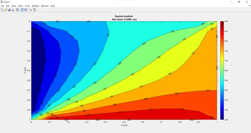
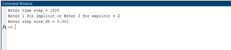
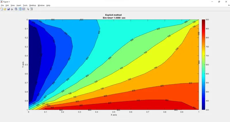
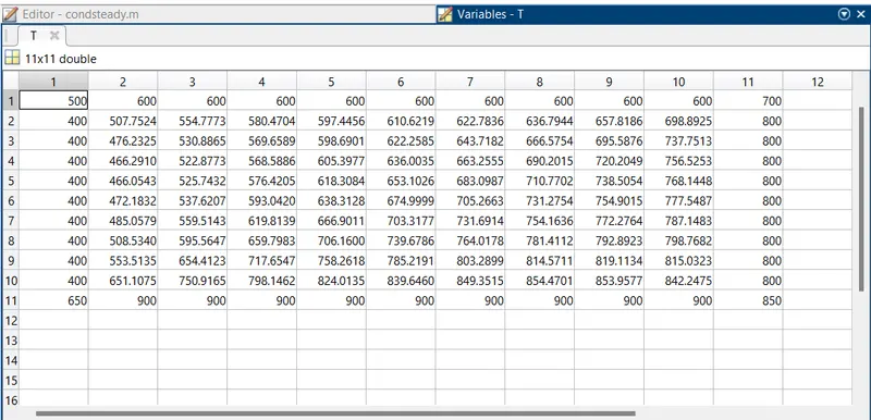
Comparison of steady state and unsteady state T values
Unsteady state
After 2.5 sec (explicit)
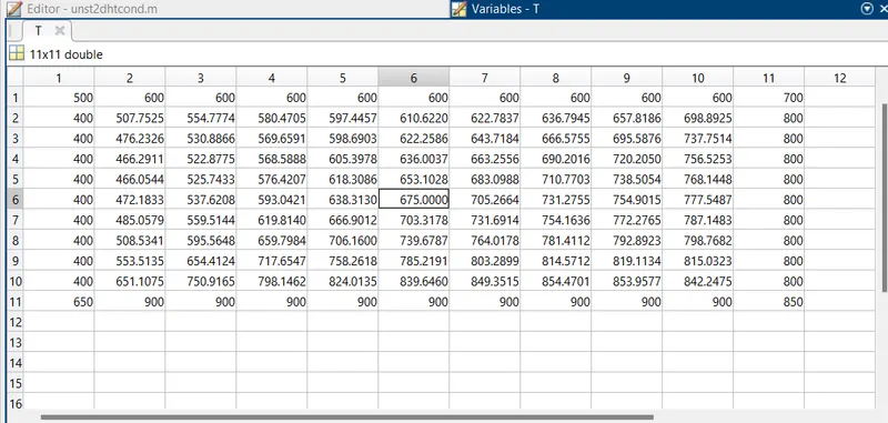
Steady state
DISCUSSION
- As all cases are observed for final steady solution, the temperature plots are same.
- The SOR method is better to get the solution faster compared to Gauss Seidel and Jacobi.
- The explicit method is easy to form, but stability needs to be checked with CFL.
- The implicit method needs iterative solver, where explicit gives the direct solution.
- Implicit methods are difficult to form but stability make it an attractive choice.
- The CFL best time step is selected in the explicit method to get the stable solution.
- The optimum value of successive over-relaxation parameter is selected based on trial and error method
- For stable solution in explicit method
k x + k y ≤ 0.50 - It is observed that after some time the unsteady state attains steady state and it gives the plot and the values of T same as that of steady state