Week 5.1 - Mid term project - Solving the steady and unsteady 2D heat conduction problem

AIM: The purpose of this MATLAB-based project is to use several iterative techniques, such as the Jacobi, Gauss-Seidel, and sequential over-relaxation methods, to solve the 2D heat conduction equation for steady state and transient states.

THEORY:

The equation of heat conduction.

that is the distribution of heat in three-dimensional space and over a period of time.
The term "alpha" is used to describe the thermal diffusivity.

IMPLICIT METHOD:

The term Implicit method refers to the process of computing a dependent variable described by a system of equations, wherein a matrix is used to determine the value of the unknown. There is no need to apply stability requirements because the procedure is stable. The solution is typically guessed in order to obtain approximative values and detect mistakes. These inaccuracies are then applied to the search for alternative overriding information. The same steps are repeated until an acceptable margin of error is determined.

EXPLICIT METHOD:

To explicitly calculate an unknown quantity given a known one is called the Explicit Method. Explicit calculation refers to this type of calculation. Stability conditions are necessary for this procedure, but the result is a robust answer. When it comes to stability criteria, baby steps are what it takes to get there. With a smaller time step, the solution converges more quickly and with greater precision, but more calculations must be done in total.

Iterative solvers types:

Jacobi
Here, we update the solution once we've found all the node values, and keep doing that until we get a convergent solution by assuming the initial values at all the nodes. However, we must transform the equations into a diagonally dominant matrix in order to use this approach.

Guass Siedel
In this iteration, rather than waiting for the first cycle to finish before assuming the values found in the Jacobi iteration, we jump right into the following equation.

successive over relaxation
This strategy improves upon the previous two methods. As an added bonus, we leverage the relaxation factor to make things easier. In our calculations, we assume that the relaxation factor is more than 1 but less than 2.

PROCEDURE:

1.First of all we take n number of nodes along x and y axis as nx and ny . Distance between two nodes along x and y axis are

dx and dy. we take temperature at each point is 300k and then take boundary conditions like top and bottom temperature are

600k and 900k and left and right are 400k and 800k.

2.We take two copy of initial conditions of temperature, T as T_old and T_prev.Take a random value of error is 9e^9 and tolerance is 1e^-4 so as error should be greater than tolrance as we have to reduce error value up to tolerance so as to achieve perfection from imperfection.Also taking the value of omega as 1.2 , if we incraese omega more so we mayface more iteration thus incorporating wrong result.

3.we have to adopt a iterative_solver (a variable)to check this method for three formulas as jacobi,gauss-seidal and sor.

Vary the iterative_solver from 1 to 3 and check each formula by if-else condition.

4.In previous its discussed that we should decrease error upto level of tolerance so we adopt a while loop where error>tolerance.Then as its a 2D problem so we have to take two for loop as i & j and vary it from 2 to (n-1) as boundary

conditions are known.

5.After for loops we are updating error value as maximum difference of T_old and newly derived T. we have to update

T_old=T as the newly derived T will be T_old in the loop for the next iteration. In each loop we have to take iteration value

before while loop and increment it by "itreration=iteration+1" before while loop finishes.These all are done at each iterative_solver.

6.We are taking x,y command as 2d form by meshgrid command and plot it by contourf command.We are taking a column like entity to show how the colors are distributed by colorbar command , we can make different types of shades of color by

colormap command.we are pointing sizes of each plot by clabel command.

7.After declaring title_method by sprintf we are taking it as title of the plot.

8.At iterative_solver=2 before while loop we are taking T_old=T_prev, as the T_old should be first value before iterative_solver=1 ,so that it can start iteration from the first T_old value otherwise T_old value will be taken after it had been

iterated at the end of the iterative_solver=1. same is done for the iterative_solver=3.

PROGRAM CODE:

for the steady state:

% steady state
clear all
close all
clc

% input
% L = 1
nx = 20;
ny = 20;
x = linspace(0,1,nx);
y = linspace(0,1,ny);
dx = x(2) - x(1);
dy = y(2) - y(1);

% Boundary condition
t = 300*ones(nx,ny);
t(:,1) = 400;
t(1,:) = 600;
t(:,nx) = 800;
t(ny,:) = 900;

% define temperature at the cornor
t(1,1) = 500;
t(1,ny) = 700;
t(nx,1) = 650;
t(nx,ny) = 850;

dt = 1e-2; %time step
told = t;

error = 100;
tol = 1e-4;
k = 2*(dx^2+dy^2)/(dx^2*dy^2);
method = input('Iterative method = ');

%jacobi iterative method
if (method==1)
    tic;
    jacobi = 1;
    while(error>tol)
        for i = 2:(nx-1)
            for j = 2:(ny-1)
                t(i,j) = (((told(i-1,j)+told(i+1,j))/(dx^2))+((told(i,j+1)+told(i,j-1))/(dy^2)))/k;
            end
        end
        error = max(max(abs(t-told)));
        told = t;
        jacobi = jacobi+1;
        time_taken = toc;
    end
    %plotting    
    figure(1)
    contourf(x,y,t,'ShowText','on');
    colormap(jet);
    colorbar;
    xlabel('X')
    ylabel('Y')
    text1 = sprintf('number of iteration = %d', jacobi);
    text2 = sprintf('simulation time = %f', time_taken);
    title({'Steady state heat conduction profile by jacobi'; text1; text2});
end

% Gauss seidel iterative method

if (method==2)
    tic;
    gs = 1;
    while(error>tol)
        for i = 2:(nx-1)
            for j = 2:(ny-1)
                t(i,j) = (((t(i-1,j)+told(i+1,j))/(dx^2))+((told(i,j+1)+t(i,j-1))/(dy^2)))/k;
            end
        end
        error = max(max(abs(t-told)));
        told = t;
        gs = gs+1;
        time_taken = toc;
    end
    %plotting    
    figure(2)
    contourf(x,y,t,'ShowText','on');
    colormap(jet);
    colorbar;
    xlabel('X')
    ylabel('Y')
    text1 = sprintf('number of iteration = %d', gs);
    text2 = sprintf('simulation time = %f', time_taken);
    title({'Steady state heat conduction profile by gauss seidel'; text1; text2});
end

% SOR iterative method
if (method==3)
    tic;
    sor = 1;
    omega = 1.4;
    while(error>tol)
        for i = 2:(nx-1)
            for j = 2:(ny-1)
                term1 =(t(i-1,j)+told(i+1,j))/(dx^2);
                term2 =(told(i,j+1)+t(i,j-1))/(dy^2);
                t(i,j) = ((told(i,j)*(1-omega)))+(omega*(term1+term2))/k;
            end
        end
        error = max(max(abs(t-told)));
        told = t;
        sor = sor+1;
        time_taken = toc;
    end
    %plotting    
    figure(3)
    contourf(x,y,t,'ShowText','on');
    colormap(jet);
    colorbar;
    xlabel('X')
    ylabel('Y')
    text1 = sprintf('number of iteration = %d', sor);
    text2 = sprintf('simulation time = %f', time_taken);
    title({'Steady state heat conduction profile by successive over relaxation'; text1; text2});
end

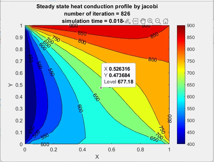
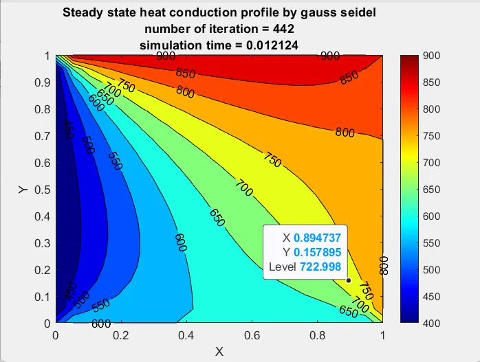
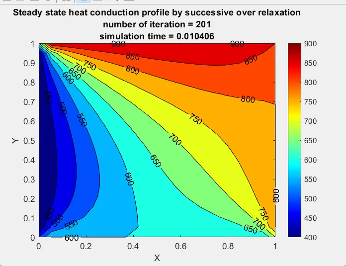
OUTPUT:

for the transient state implicite method:

% TRANSIENT STATE IMPLICIT METHOD
clear all
close all
clc

% initial condition
% L = 1
nx = 20;
ny = 20;
x = linspace(0,1,nx);
y = linspace(0,1,ny);
dx = x(2) - x(1);
dy = y(2) - y(1);

% Boundary condition
t = 300*ones(nx,ny);
t(:,1) = 400;
t(1,:) = 600;
t(:,nx) = 800;
t(ny,:) = 900;

% define temperature at the cornor
t(1,1) = 500;
t(1,ny) = 700;
t(nx,1) = 650;
t(nx,ny) = 850;

nt = 300; % No.of steps

dt = 1e-2; %time step
told = t;
tprev_dt = told;

error = 100;
tol = 1e-4;
alpha = 1; % Thermal diffusivity
k1 = alpha*dt/(dx^2);
k2 = alpha*dt/(dy^2);

method = input('Iterative method = ');

% jacobi method
if (method==1)
    tic;
    jacobi = 1;
    for p = 1:nt
        error =100;
        while(error>tol)
            for i = 2:(nx-1)
                for j = 2:(ny-1)
                    term1 = (1+(2*k1)+(2*k2))^-1;
                    term2 = k1*term1;
                    term3 = k2*term1;
                    h = (told(i-1,j)+told(i+1,j));
                    v = (told(i,j+1)+told(i,j-1));
                    t(i,j) = ((tprev_dt(i,j)*term1)+(h*term2)+(v*term3));
                end
            end
        
            error = max(max(abs(t-told)));
            told = t;
            jacobi = jacobi+1;
         end
         tprev_dt = t ;
    end
    time_taken = toc;

%plotting    
figure(1)
contourf(x,y,t,'ShowText','on');
colormap(jet);
colorbar;
xlabel('X')
ylabel('Y')
text1 = sprintf('number of iteration = %d', jacobi);
text2 = sprintf('simulation time = %f', time_taken);
title({'Transient state heat conduction profile Implicit-Jacobi'; text1; text2});
end

% gauss seidel method
if (method==2)
    tic;
    gauss = 1;
    for p = 1:nt
        error =100;
        while(error>tol)
            for i = 2:(nx-1)
                for j = 2:(ny-1)
                    term1 = (1+(2*k1)+(2*k2))^-1;
                    term2 = k1*term1;
                    term3 = k2*term1;
                    h = (t(i-1,j)+told(i+1,j));
                    v = (told(i,j+1)+t(i,j-1));
                    t(i,j) = ((tprev_dt(i,j)*term1)+(h*term2)+(v*term3));
                end
            end
        
            error = max(max(abs(t-told)));
            told = t;
            gauss = gauss+1;
         end
         tprev_dt = t; 
    end
    time_taken = toc;

    %plotting    
    figure(2)
    contourf(x,y,t,'ShowText','on');
    colormap(jet);
    colorbar;
    xlabel('X')
    ylabel('Y')
    text1 = sprintf('number of iteration = %d', gauss);
    text2 = sprintf('simulation time = %f', time_taken);
    title({'Transient state heat conduction profile Implicit-Gauss-seidel'; text1; text2});
end

% successive over relaxation method


if (method==3)
    tic;
    sor = 1;
    omega = 1.2; % Over relaxation factor
    for p = 1:nt
        error =100;
        while(error>tol)
            for i = 2:(nx-1)
                for j = 2:(ny-1)
                    term1 = (1+(2*k1)+(2*k2))^-1;
                    term2 = k1*term1;
                    term3 = k2*term1;
                    h = (t(i-1,j)+told(i+1,j));
                    v = (told(i,j+1)+t(i,j-1));
                    t(i,j) = (told(i,j)*(1-omega))+(omega*((tprev_dt(i,j)*term1)+(h*term2)+(v*term3)));
                end
            end
        
            error = max(max(abs(t-told)));
            told = t;
            sor = sor+1;
         end
         tprev_dt = t ;
    end
    time_taken = toc;

%plotting    
figure(3)
contourf(x,y,t,'ShowText','on');
colormap(jet);
colorbar;
xlabel('X')
ylabel('Y')
text1 = sprintf('number of iteration = %d', sor);
text2 = sprintf('simulation time = %f', time_taken);
title({'Transient state heat conduction profile Implicit-SOR'; text1; text2});
end

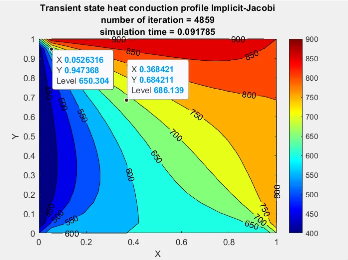
OUTPUT:

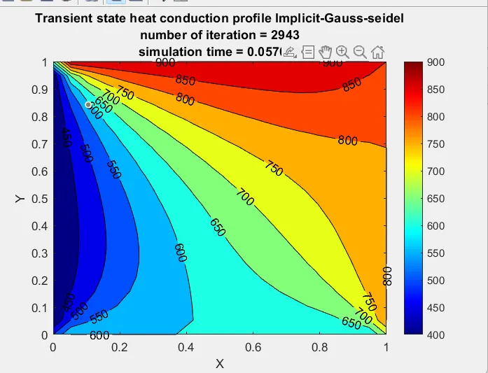
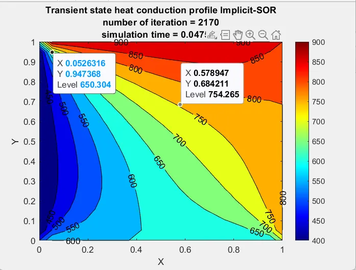
for transient state explicit method:

% TRASIENT STSTE EXPLICIT METHOD
clear all
close all
clc

%inputs data
%L = 1
nx = 10;
ny = 10;
nt = 300; % No.of steps
x = linspace(0,1,nx);
y = linspace(0,1,ny);
dx = x(2) - x(1);
dy = y(2) - y(1);

% initial temperature

t = 300*ones(nx,ny);  
t(:,1) = 400;
t(1,:) = 600;
t(:,ny) = 800;
t(nx,:) = 900;

% defining the temperature at corner points

t(1,1) = 500;
t(nx,ny) = 850;
t(1,ny) = 700;
t(nx,1) = 650;

dt = 0.01; %time step
told=t;
alpha = 0.3; % Thermal diffusivity

k1 = (alpha*dt)/(dx^2);
k2 = (alpha*dt)/(dy^2);
CFL = alpha*dt/(dx^2);

% running for loop

tic;
explicit = 1;
for p = 1:nt
    for i = 2:(nx-1)
        for j = 2:(ny-1)
            term1 = (told(i-1,j)-2*told(i,j)+told(i+1,j));
            term2 = (told(i,j-1)-2*told(i,j)+told(i,j+1));
            t(i,j) = ((told(i,j))+(k1*term1)+(k2*term2));
        end
    end
        
    told = t;
    explicit = explicit+1;
end

time_taken = toc;
  
%Plotting   
figure(1)
contourf(x,y,t,'ShowText','on');
colormap(jet);
colorbar;
xlabel('X')
ylabel('Y')
text1 = sprintf('time = %d', dt*nt);
text2 = sprintf('simulation time = %f', time_taken);
title({'Transient state heat conduction profile Explicit'; text1; text2});

OUTPUT:

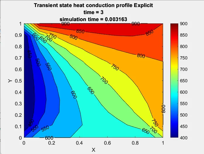
CONCLUSION:

From the above graphs we can say that when we compare steady and unsteady state , steady state is the most successful as it takes least number of iterations and least time to compute. SOR iteration is the most effective among the three method as it took less number of iterations from both the ways. For transient equations time required to solve is more compared to steady state equations.So, therefore it is recommended to solve the 2D heat conduction equation with steady state conditions.