Week 5.1 - Mid term project - Solving the steady and unsteady 2D heat conduction problem

AIM: The purpose of this MATLAB-based project is to use several iterative techniques, such as the Jacobi, Gauss-Seidel, and sequential over-relaxation methods, to solve the 2D heat conduction equation for steady state and transient states.

Problem Definition:

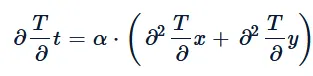
Pde provides a definition for the equation of heat conduction.

that is the distribution of heat in three-dimensional space and over a period of time.
The term "alpha" is used to describe the thermal diffusivity.

Approaches Taken

To explicitly calculate an unknown quantity given a known one is called the "Explicit Method." Explicit calculation refers to this type of calculation. Stability conditions are necessary for this procedure, but the result is a robust answer. When it comes to stability criteria, baby steps are what it takes to get there. With a smaller time step, the solution converges more quickly and with greater precision, but more calculations must be done in total.

The term "implicit method" refers to the process of computing a dependent variable described by a system of equations, wherein a matrix is used to determine the value of the unknown. There is no need to apply stability requirements because the procedure is stable. The solution is typically guessed in order to obtain approximative values and detect mistakes. These inaccuracies are then applied to the search for alternative overriding information. The same steps are repeated until an acceptable margin of error is determined.

Iterative solvers are employed in the process of resolving dependent variables. And those are:-

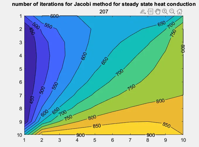
Iterative solver by Jacobi
Here, we update the solution once we've found all the node values, and keep doing that until we get a convergent solution by assuming the initial values at all the nodes. However, we must transform the equations into a diagonally dominant matrix in order to use this approach.

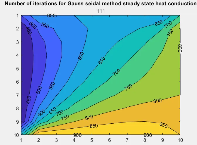
Problem-Solver Guass Siedel
In this iteration, rather than waiting for the first cycle to finish before assuming the values found in the Jacobi iteration, we jump right into the following equation.

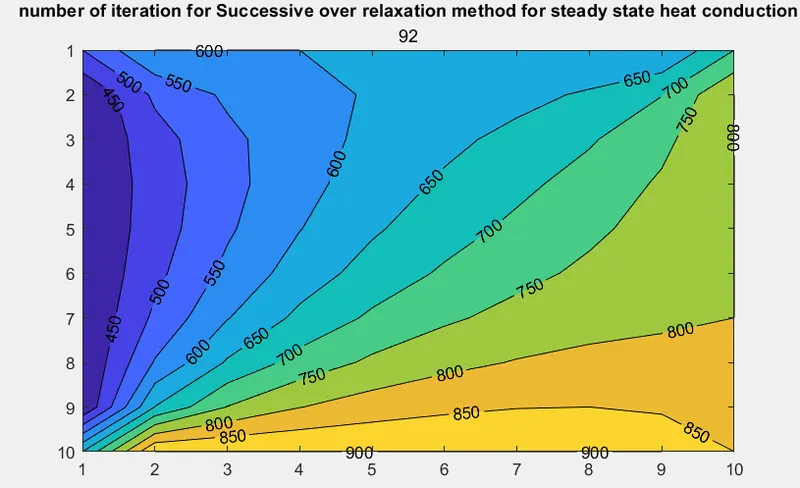
Solver success over relaxation
This strategy improves upon the previous two methods. As an added bonus, we leverage the relaxation factor to make things easier. In our calculations, we assume that the relaxation factor is more than 1 but less than 2.

Transient state of eqation in 2D

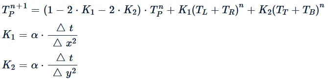
solving 2D transient heat conduction equation explicitly we get

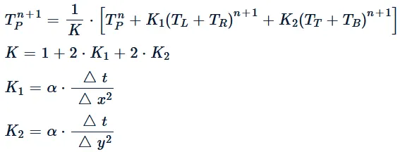
Solving for implicitly we get

The temperature does not change in a steady state, so Steady state equation:

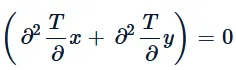
Using various iterative techniques to solve the steady state 2D problem

Conditions of the boundary

We define bottom, top, left, and right boundary temperatures in a 10 by 10 matrix as independent variables. together with a proposed baseline temperature of 300K.

Main code:

• Using separate function files, the same Matlab code can be used for both steady and unstable conditions.
• When programming, the domain is the surface of the area (1 m by 1 m).
• Separated into 10 horizontal and vertical nodes.
• If you remember the explicit condition, you can find constant values like alpha and the "data" for each time step.
• When writing code, the relaxation factor for SOR is also taken into account.

close all
clear all
clc

% space domain
nx=10;
ny=nx;

% length of domain
L=1;

% defining space domain
x= linspace(0,L,nx);
y= linspace(0,L,ny);


dx = L/(nx-1);
dy = L/(ny-1);
% guess temperature 300K
T= 300*ones(nx,ny);

% Initia boundary conditions at left and right
T(1:end,1) = 400;
T(1:end,end) = 800;


% Initia boundary conditions at bottom and top
T(end,1:end) = 900;
T(1,1:end) = 600;


%average values of T at corner boundaries
T(1,1) = 500;
T(end,1) = 650;
T(1,end) = 700;
T(end,end) = 850;

% Tolerence
tol= 1e-4;

% copy of temperature
told=T;
t_initial=T;

%Coefficient for steady state equation
k = 2*((dx^2)+(dy^2))/((dx^2)*(dy^2));

%diffusivity co-efficient 
alpha = 1.4;

%Relaxation Factor
a = 1.1;

% Calculation of time step
dt = (0.5)/((alpha/(dx^2))+(alpha/(dy^2)));

% Co-efficient  multipied for x diffuse term
k1 = dt*alpha/dx^2;
% Co-efficient  multipied for y diffuse term
k2 = dt*alpha/dy^2;

%relaxation factor for transiet heat conduction
a1 = 1.15;

%Function to calculate the temperature of Steady state using jacobi iterative solver
[error_j,itr_jacobi, time_jacobi] = jacobi_steadystate(nx,ny,T,told,k,dx,dy,tol);


%Function to calculate the temperature of Steady state using Gauss Seidal iterative solver    
[error_gs,itr_gs] = gauss_steadystate(nx,ny,T,told,k,dx,dy,tol);


%Function to calculate the temperature Steady state using Successive over relaxation iterative solver    
[error_sor,itr_sor] = sor_steadystate(nx,ny,T,told,k,dx,dy,tol,a); 


%Function to calculate the temperature of Transient heat conduction explicitly    
[error_dt,iter_dt]=transient_heat_cond(nx,ny,k1,k2,told,T,tol,dt);   


%Function to calculate the temperature of Unsteady state using jacobi iterative solver
[error_jac,iter_jac]=transient_heat_cond_jacobi(nx,ny,k1,k2,told,T,tol,t_initial,dt);


%Function to calculate the temperature of Unsteady state using Gauss Seidal iterative solver
[error_gs_imp,iter_gs_imp]=transient_heat_cond_gs(nx,ny,k1,k2,told,T,tol,t_initial,dt);


%Function to calculate the temperature of Unsteady state using Successive over relaxation iterative solver
[error_sor_gs_imp,iter_sor_gs_imp]=transient_heat_cond_sor_gs(nx,ny,k1,k2,told,T,tol,t_initial,a1,dt);

Explanation of Main Code

• Choosing the number of grid points in the x and y space In this case, there are 10 grid points along the x and y axes.
• Setting the length of the domain in x and y equals 1 in this case.
• Defining the space domain for the specified length and grid points.
• In the x and y space domains, grid spacing is worked out.
• The temperature guess value for the number of defined grid points is 300K.
• Using the boundary conditions from the problem.
• The accuracy of the solution is measured by comparing the approximate solution that was found to the tolerance value. This makes sure that the converged solution is within the range of accuracy that was set.
• In told and t initial, a copy of the initial temperature matrix is made. This copy is used when explicitly and implicitly figuring out the temperature at n+1 time steps.
• Here alpha is approximated to be 1.4.
• The temperature at the n+1 time step is computed in two ways: first, using an iterative solution specific to steady-state heat conduction; second, using an explicit technique specific to unsteady heat conduction.

Explanation of FUNCTIONS in Main Code

• In functions, the error variable is always set to an error dummy to ensure that the while loop condition is always met.
  
• There are two for loops inside the while statement, allowing us to generate data for all x and y coordinates and the absolute value of the error.
  
• At the ending of the for loop, we update the value by assigning told to t.
  
• The number of iterations is calculated by assigning a value of +1 to the iterative value.
  
• When we talk about transient and steady-state formulas, we're referring to the formulas used by "T" to store temperature data.
  
• After all, we draw the desired data plot's contours while the loop is running and at the end of the loop.
  
• In the transitional condition, the time marching step is added as nt = T/dt. To do this, we place a for loop before the while loop and then assign =T at the end of the while loop, so that the result of the first iteration is used for the following time step.

FUNCTION CODES

Steady state jacobi method

function [error_j,itr_jacobi, time_jacobi] = jacobi_steadystate(nx,ny,T,told,k,dx,dy,tol)


% defining iteration
itr_jacobi=0;

% dummy error value 
error_j = 9e9;

tic
%convergence loop
while (error_j > tol)

    %iteration loop
    for i= 2:nx-1
        
        for j= 2:ny-1
            % formula to calculate the temperature
                TL = told(i-1,j);
                TR = told(i+1,j);
                TB = told(i,j-1);
                TT = told(i,j+1);
                
                term1 = (TL +TR)/(dx^2);
                term2 = (TB +TT)/(dy^2);
                T(i,j)= (term1 + term2)* 1/k;
        end
    end
    error_j= max(max(abs(told - T)));
    told= T;

    % updating iteration  
    itr_jacobi= itr_jacobi+1;
end
time_jacobi=toc;
figure(1)
[C,h]=contourf(T);
%Labelling the plot here C reperesents the temperature values and h rotates the temperature values as it moves.
 clabel(C,h);
 axis ij;
title('number of iterations for Jacobi method for steady state heat conduction',itr_jacobi);

end

Steady state Guass siedel method

function [error_gs,itr_gs] = gauss_steadystate(nx,ny,T,told,k,dx,dy,tol)

% defining iteration
itr_gs=0;
% dummy error value 
error_gs= 9e9;

%convergence loop
while (error_gs > tol)
    %iteration loop
    for i= 2:(nx-1)
        for j= 2:(ny-1)
            % formula to calculate the temperature
                TL = T(i-1,j);
                TR = told(i+1,j);
                TB = T(i,j-1);
                TT = told(i,j+1);
                
                term1= (TL +TR)/dx^2;
                term2 = (TB +TT)/dy^2;
                T(i,j)= (1/k)*(term1 + term2);
        end
    end
    error_gs= max(max(abs(told - T)));
    told=T;
    % iteration updation 
    itr_gs= itr_gs+1;
end
  % Plot representing the converged results.
figure(2)
[C,h]=contourf(T);
%Labelling the plot here C reperesents the temperature values and h rotates the temperature values as it moves.
clabel(C,h);
axis ij;
title('Number of iterations for Gauss seidal method steady state heat conduction',itr_gs)
end

Steady state Sor method

function [error_sor,itr_sor] = sor_steadystate(nx,ny,T,told,k,dx,dy,tol,a)
% defining iteration
itr_sor=0;
% dummy error value 
error_sor= 9e9;

%convergence loop
while (error_sor > tol)
    %iteration loop
    for i= 2:(nx-1)
        for j= 2:(ny-1)
            % formula to calculate the temperature
                TL = T(i-1,j);
                TR = told(i+1,j);
                TB = T(i,j-1);
                TT = told(i,j+1);
                
                term1 = (TL +TR)/dx^2;
                term2 = (TB +TT)/dy^2;
                T(i,j)= (told(i,j))*(1-a) + a*((term1 + term2)/k);
               
        end
    end
    error_sor= max(max(abs(told - T)));
    told=T;
    % iteration updation 
    itr_sor= itr_sor+1;
end
% Plot representing the converged results.
  figure(3)
  [C,h]=contourf(T);
  %Labelling the plot here C reperesents the temperature values and h rotates the temperature values as it moves.
  clabel(C,h);
  axis ij;
  title('number of iteration for Successive over relaxation method for steady state heat conduction', itr_sor)

end

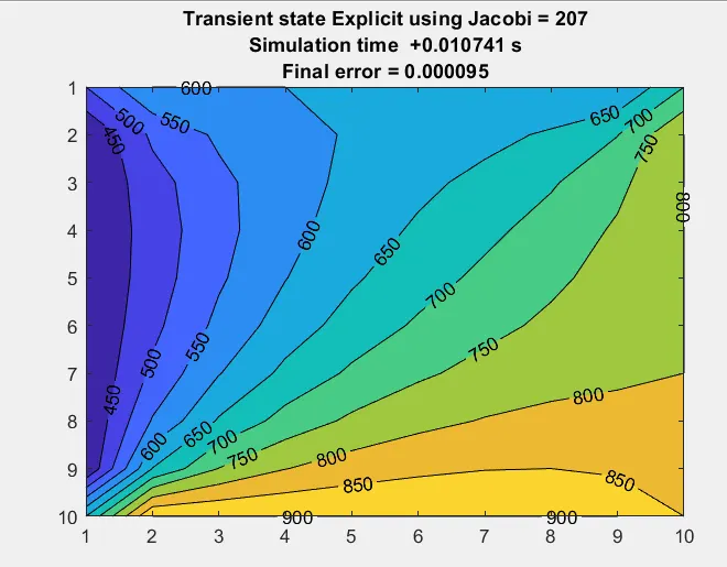
Unsteady state Explicit method

The difference from the previous example is adding a time-marching loop before the while for n+1 time steps.

function [error_dt,iter_dt]=transient_heat_cond(nx,ny,k1,k2,told,T,tol,dt)

    %dummy error
    error_dt = 9e9;
    %defining iteration variable to store and display the number of iterations computed for the values to converge.
   
    iter_dt =0;
    %convergence loop time marching
    
    nt= T/dt;
    tic
    for m= 1:nt
    while (error_dt>tol)
            
            %Iteration loop
     for i = 2:nx-1
         for j = 2:ny-1
             
              term1 = told(i-1,j)-2*told(i,j)+told(i+1,j);% temperature values in x direction
              term2 = told(i,j-1)-2*told(i,j)+told(i,j+1);% temperature values in y direction

                %Formula to calculate the temperature at each grid point
                    

                    T(i,j)= told(i,j)+k1*term1+k2*term2;      
                    
                end
            end

           %error for each iteration
        
            error_dt = max(max(abs(told-T)));
            
            %updating the temperature values for the next iteration. 
            told = T;
            
           %incrementing iteration variable by 1 to display the no. of iterations taken for the solution to converge.
           
           iter_dt = iter_dt+1;
           


    end 
    told=T;
    end
    time1=toc;

           %Plot representing the converged results.
           figure(4)       
           [C,h]=contourf(T);

           %Labelling the plot here C reperesents the temperature values and h rotates the temperature values as it moves.
           clabel(C,h);
           axis ij

           %title('Number of iterations using transient heat conduction explicitly',iter_dt);
           title_text1 = sprintf('Transient state Explicit using Jacobi = %d', iter_dt);
        title_text2 = sprintf('Simulation time  +%f s', time1);
        title_text3 = sprintf('Final error = %f' , error_dt);
        title({title_text1; title_text2;title_text3});
end

Function for Unsteady state using jacobi method.

• Transient state problems require additional timesteps to be solved.
• The first while loop does a steady-state solution check by determining the delta between two successive temperature readings and two successive tolerance readings.
• After the temperature has converged for a specific time step, the process will continue indefinitely.
• The "for" loop determines the time marching in nt time steps prior to entering the while loop.
• As a last step, we update T with each new time step by assigning told.
• Tic toe is used to determine how long an iteration takes to solve.

function [error_jac,iter_jac] = transient_heat_cond_jacobi(nx,ny,k1,k2,told,T,tol,t_initial,dt)

    % dummy error
    error_jac=9e9;
    error_f = 9e9;

   %defining iteration variable to store and display the number of
   %iterations computed for the values to converge.
    iter_jac=0;

     %time marching
    nt= T/dt;
    tic

    for m= 1:nt
    %While loop to stop iterations when the temperature values converge while computing for different time steps.

    while (error_f>tol)
        
        %Convergence loop each time step
        while (error_jac>tol)

                %Iteration loop
                for i = 2:nx-1

                    for j = 2:ny-1
                        
                        %Co-efficient obtained while deriving for transient heat conduction equation
                        term1= (1+(2*k1)+(2*k2))^-1;

                        %k1 and k2 represent the cfl value for x and y domain repectively
                       
                        term2 = told(i-1,j)+told(i+1,j);% temperature values in x direction
                        term3 = told(i,j-1)+told(i,j+1);% temperature values in y direction

                        %Formula to calculate the temperature at each grid point
                        T(i,j)= (t_initial(i,j)*term1)+(term1*k1*term2)+(term1*k2*term3);


                    end
                end

                %error for each iteration
              
                error_jac = max(max(abs(told-T)));
                %updating the temperature values for the next iteration. 
                told = T;
                
                %incrementing iter variable by 1 to display the no. of iterations taken for the solution to converge.
              
                iter_jac = iter_jac+1;

 
        end 
      
      % error defined to obtain desired accuracy for the convergenc rate.
      error_f = max(max(abs(t_initial-T)));
      t_initial = T; 
      %Reseting the error value for the covergence loop to compute for the next time step.
      
      error_jac = 9e9;

    end
    told=T;
    end
    time2=toc;
                %Plot representing the converged results.
                figure(5)       
               [C,h]=contourf(T);
               %Labelling the plot here C reperesents the temperature values and h rotates the temperature values as it moves.
               clabel(C,h)
               axis ij
               %title('Number of iterations for implicit Jacobi',iter_jac);
               title_text1 = sprintf('Transient state Implicit using Jacobi = %d', iter_jac);
        title_text2 = sprintf('Simulation time  +%f s', time2);
        title_text3 = sprintf('Final error = %f' , error_f);
        title({title_text1; title_text2;title_text3});

end

Transient Guass siedel method

function [error_gs_imp,iter_gs_imp]=transient_heat_cond_gs(nx,ny,k1,k2,told,T,tol,t_initial,dt)

    %Definition of dummy error
    error_f = 9e9;
    error_gs_imp =9e9;

   %defining iteration variable to store and display the number of iterations computed for the values to converge
   
    iter_gs_imp=0;

     %time marching
    nt= T/dt;
    tic
    for m= 1:nt

    %While loop to stop iterations when the temperature values converge whle computing for different time steps.
    while(error_f >tol)
        
        %Convergence loop each time step
        while (error_gs_imp>tol)

                %Iteration loop
                for i = 2:nx-1

                    for j = 2:ny-1
                        
                        %Co-efficient obtained while deriving for transient heat conduction equation
                        term1= (1+(2*k1)+(2*k2))^-1;

                        %k1 and k2 represent the cfl value for x and y domain repectively.
                        
                        term2 = T(i-1,j)+told(i+1,j);%  temperature values in x direction
                        term3 = T(i,j-1)+told(i,j+1);%  temperature values in y direction

                        %Formula to calculate the temperature at each grid point
                        
                        T(i,j)= (t_initial(i,j)*term1)+(term1*k1*term2)+(term1*k2*term3);


                    end
                end

                %error for each iteration
               
                error_gs_imp =max( max(abs(told-T)));
                
                %updating the temperature values for the next iteration.  
                told = T;
                
               %incrementing iter variable by 1 to display the no. of iterations taken for the solution to converge.
               
               iter_gs_imp = iter_gs_imp+1;

 
        end 
      
      % error defined to obtain desired accuracy for the convergenc rate.
      error_f = max(max(abs(t_initial-T)));

      %Updating the previous temperature values to computed values.
      t_initial = T; 

      %Reseting the error value for the covergence loop to compute for the next time step.
      
      error_gs_imp = 9e9;

    end
    told=T;
    end
      time3=toc;
      %Plot representing the converged results.
                figure(6)       
               [C,h]=contourf(T);
               %Labelling the plot here C reperesents the temperature values and h rotates the temperature values as it moves.
               clabel(C,h)
               axis ij
               %title('Number of iterations for implicit Gauss seidal',iter_gs_imp);
                title_text1 = sprintf('Transient state Implicit using Gauss SIEDEL = %d', iter_gs_imp);
        title_text2 = sprintf('Simulation time  +%f s', time3);
        title_text3 = sprintf('Final error = %f' , error_f);
        title({title_text1; title_text2;title_text3});


end

Transient SOR method

function [error_sor_gs_imp,iter_sor_gs_imp]=transient_heat_cond_sor_gs(nx,ny,k1,k2,told,T,tol,t_initial,a1,dt)
        
        %dummy error
        error_f = 9e9;
        error_sor_gs_imp = 9e9;

        %defining iteration variable to store and display the number of iterations computed for the values to converge.
         iter_sor_gs_imp =0;

        %time marching
        nt= T/dt;
    tic
    for m= 1:nt

    %While loop to stop iterations when the temperature values converge while computing for different time steps.
        while (error_f>tol)
        
        %Convergence loop each time step
        
        while (error_sor_gs_imp>tol)

                %Iteration loop
                for i = 2:nx-1

                    for j = 2:ny-1
                        %Co-efficient obtained while deriving for transient heat conduction equation
                        term1= (1+(2*k1)+(2*k2))^-1;
                        term2 = T(i-1,j)+told(i+1,j);% temperature values in x direction
                        term3 = T(i,j-1)+told(i,j+1);% temperature values in y direction

                        %Formula to calculate the temperature at each grid point
                        
                        T(i,j)= (t_initial(i,j)*term1)+(term1*k1*term2)+(term1*k2*term3);

                        %Successive over relaxation Formula to calculate the temperature at each grid point.
                        
                        T(i,j)= (told(i,j))*(1-a1)+ a1*T(i,j);
                        


                    end
                end
                
               %error for each iteration
               
               error_sor_gs_imp = max(abs(told - T));
               
               %updating the temperature values for the next iteration.
               told = T;
               
                %incrementing iter variable by 1 to display the no. of
               %iterations taken for the solution to converge.
               iter_sor_gs_imp = iter_sor_gs_imp+1;

 
        end 
        
      %error defined to obtain desired accuracy for the convergenc rate.
      error_f = max(max(abs(t_initial-T)));

      %Updating the previous temperature values to computed values.
      t_initial = T;

      %Reseting the error value for the covergence loop to compute for the next time step.
      error_sor_gs_imp = 9e9;
      
    end
    told=T;
    end
    time4=toc;
               %Plot representing the converged results.
               figure(7)       
               [C,h]=contourf(T);

               %Labelling the plot here C reperesents the temperature values and h rotates the temperature values as it moves.
               clabel(C,h)
               axis ij

               %title('Number of iteration for implicit SOR',iter_sor_gs_imp);
                title_text1 = sprintf('Transient state Implicit using SOR = %d', iter_sor_gs_imp);
                title_text2 = sprintf('Simulation time  +%f s', time4);
                title_text3 = sprintf('Final error = %f' , error_f);
                title({title_text1; title_text2;title_text3});

               

end

Results:

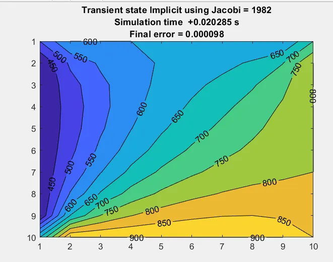
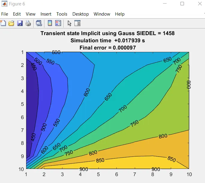
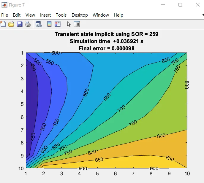
CONCLUSION

• The implicit approach can be utilised to find solutions to situations when converged results are required in a shorter amount of time spent doing computations because it is unconditionally stable. When the size of the timestep is increased, the convergence rate also increases, which means that the system reaches a steady state in a shorter amount of time. Count of previous iterations
• The explicit method is a time-accurate method since it is governed by stability criteria; if these criteria are not satisfied, it leads to an unstable solution and necessitates further iterations to reach a steady state.
• Nonetheless, the above-provided code specifies a consistent step size, so we know this is a reliable requirement.
• Therefore, the explicit leads to a higher rate of convergence, and as the time step becomes smaller, the number of repetitions of the implicit scheme grows, resulting in a slower rate of convergence.