Week 5.1 - Mid term project - Solving the steady and unsteady 2D heat conduction problem

CHALLENGE - 5.1 : Solving the Steady and Unsteady 2D Heat Conduction Problem

AIM:

To write a Matlab program to solve and plot the contours of steady and unsteady 2D Heat conduction probelm.

OBJECTIVE:

1. To write a Matlab program to solve steady and unsteady 2D Heat conduction probelm by adopting different methods.
2. To plot the temperature contour of the same for all the available methods.
3. To compare the results obtained for each case.

THEORY:

1. Governing differential equation of two dimensional steady state heat conduction is:

`(del^2T)/(delx^2)+(del^2T)/(dely^2) = 0`

Upon discretizing the above equation by using Central difference method we get:

`(T_(i-1,j)-2T_(i,j)+T_(i+1,j))/(trianglex^2)+(T_(i,j-1)-2T_(i,j)+T_(i,j+1))/(triangley^2)= 0`

Upon re-arranging the above equation we get

`T_(i,j) = 1/K((T_(i-1,j)+T_(i+1,j))/(trianglex^2))+1/K((T_(i,j-1)+T_(i,j+1))/(triangley^2))= 0`

Where `K = 2((trianglex^2+triangley^2)/(trianglex^2**triangley^2))`

Solve the above equation using different iterative methods such as

• Jacobi Iteration Method

Here use the old value of Temperature for evaluting the Temperature at next time step.

• Gauss Seidel Iteration Method

Here use the most updated value of Temperature for evaluting the Temperature at next time step.

• Successive Over Relaxation Method (SOR)

Here use the most updated value of Temperature and a relaxation factor(w) for evaluting the Temperature at next time step.

i.e., `T_(i,j)=(1-w)T_(old)+w(T_("Gauss Seidel"))`

when w < 1 under relaxation

w>1 over relaxation

w = 1 same as G.S method.

2. Governing differential equation of two dimensional un-steady state heat conduction is:

`(delT)/(delt)=alpha((del^2T)/(delx^2)+(del^2T)/(dely^2))`

Upon discretizing the above equation by using Explicit Method we get:

`(T_p^(n+1)-T_p^n)/(trianglet)=alpha[(T_(i-1,j)-2T_(i,j)+T_(i+1,j))/(trianglex^2)+(T_(i,j-1)-2T_(i,j)+T_(i,j+1))/(triangley^2)]^n`

Upon solving the above equation we get

`T_p^(n+1)=T_p^n+K_1[(T_(i-1,j)-2T_(i,j)+T_(i+1,j))]^n+K_2[(T_(i,j-1)-2T_(i,j)+T_(i,j+1))]^n`

Where

`K_1 = (alphatrianglet)/(trianglex^2)` & `K_2 = (alphatrianglet)/(triangley^2)`

Solve the above equation for a particular time step say 1500 time steps.

Discretise the same equation by using Implicit method we get

`(T_p^(n+1)-T_p^n)/(trianglet)=alpha[(T_(i-1,j)-2T_(i,j)+T_(i+1,j))/(trianglex^2)+(T_(i,j-1)-2T_(i,j)+T_(i,j+1))/(triangley^2)]^(n+1)`

Upon solving the above equation we get:

`T_p^(n+1)=1/(1+2K_1+2K_2)[T_p^n+K_1[(T_(i-1,j)+T_(i+1,j))]^(n+1)+K_2[(T_(i,j-1)+T_(i,j+1))]^(n+1)]`

Where

`K_1 = (alphatrianglet)/(trianglex^2)` & `K_2 = (alphatrianglet)/(triangley^2)`

Solve the above equation using different iterative methods such as

• Jacobi Iteration Method

Here use the old value of Temperature for evaluting the Temperature at next time step.

• Gauss Seidel Iteration Method

Here use the most updated value of Temperature for evaluting the Temperature at next time step.

• Successive Over Relaxation Method (SOR)

Here use the most updated value of Temperature and a relaxation factor(w) for evaluting the Temperature at next time step.

i.e., `T_(i,j)=(1-w)T_(old)+w(T_("Gauss Seidel"))`

when w < 1 under relaxation

w>1 over relaxation

w = 1 same as G.S method.

Input Conditions:

Top Boundary = 600 K

Bottom Boundary = 900 K

Left Boundary = 400 K

Right Boundary = 800 K

Inner nodes = 300 K (Initial Condition)

Number of grid points in x and y direction = 11.

Length in x and y direction = 1m.

Thermal Diffusivity = 1.5 m²/s

SOR - Relaxation Factor (w) = 1.1

Error tolerence value = 1e-4

PROCEDURE:

Procedure for matlab program for steady case is mentioned below.

1. Program is started by using the general commands clear all, close all and clc to clear and close all the pre-occupied operations of Matlab.
2. Provide the input coditions.
3. Provide a command to choose the type of solver by user.
4. Evaluate the above mentioned equation of steady state with a cascade for loop for space discretization and a while loop for absolute error criteria. Evalute the error between new value of temperature and old value till it reaches the tolerance limit.
5. Plot the contour of temperature by using contourf command and provide suitable title
6. Repeat the above steps for all the three iterative method (Jacobi, Gauss Seidel and SOR).
7. Save and Run the file.

The program which is created on Matlab for steady state condition is attached below.

% Program to solve the steady state 2D heat conduction problem

clear all
close all
clc

% Input conditions
nx = 11;
ny = 11;
lx = 1;
ly = 1;
T(1:nx, 1:nx) = 300;
T(1,1) = 650;
T(1, end) = 850;
T(end, 1) = 500;
T(end, end) = 700;
T(1, 2:(end-1)) = 900;
T(end, 2:(end-1)) = 600;
T(2:(end-1), 1) = 400;
T(2:(end-1), end) = 800;
x = linspace(0,lx,nx);
y = linspace(0,ly,ny);

% Defining the time and space step size, error and tolerance value.
T_old = T;
T_initial = T;
tol = 1e-4;
err = 9e9;
dx = lx/(nx-1);
dy = ly/(ny-1);
[xx, yy] = meshgrid(x, y);

% Command to select the type of iterative solver
prompt = 'choose iterative solver, 1 = Jacobi Method, 2 = Gauss Seidel Method, 3 =  SOR Method \n';
iterative_solver = input(prompt);


% Jacobi Method
if iterative_solver == 1
k = 2*(((dx^2)+(dy^2))/((dx^2)*(dy^2)));
iter = 1;
while(err>tol)
    for i = 2:nx-1
        for j = 2:ny-1
            Term_1 = (T_old(i-1,j)+T_old(i+1,j))/(dx^2);
            Term_2 = (T_old(i,j+1)+T_old(i,j-1))/(dy^2);
            T(i,j) = 1/k*(Term_1)+1/k*(Term_2);
        end
    end
    err = max(max(abs(T_old -T)));
    T_old = T;
    iter = iter +1;
end
[x,y]= contourf(xx,yy,T);
        colormap(jet)
        colorbar
        clabel(x,y)
        title('Temperature Contour') 
end

% Gauss seidel Method
if iterative_solver == 2
k = 2*(((dx^2)+(dy^2))/((dx^2)*(dy^2)));
iter = 1;
while(err>tol)
    for i = 2:nx-1
        for j = 2:ny-1
            Term_1 = (T(i-1,j)+T(i+1,j))/(dx^2);
            Term_2 = (T(i,j+1)+T(i,j-1))/(dy^2);
            T(i,j) = 1/k*(Term_1)+1/k*(Term_2);
        end
    end
    err = max(max(abs(T_old -T)));
    T_old = T;
    iter = iter +1;
end
[x,y]= contourf(xx,yy,T);
        colormap(jet)
        colorbar
        clabel(x,y)
        title('Temperature Contour')
end

% Gauss seidel With SOR Method
w = 1.1;   % Relaxation Factor
if iterative_solver == 3
k = 2*(((dx^2)+(dy^2))/((dx^2)*(dy^2)));
iter = 1;
while(err>tol)
    for i = 2:nx-1
        for j = 2:ny-1
            Term_1 = (T(i-1,j)+T(i+1,j))/(dx^2);
            Term_2 = (T(i,j+1)+T(i,j-1))/(dy^2);
            T(i,j) = ((1-w)*T_old(i,j))+(w*(1/k*(Term_1)+1/k*(Term_2)));
        end
    end
    err = max(max(abs(T_old -T)));
    T_old = T;
    iter = iter +1;
end
[x,y]= contourf(xx,yy,T);
        colormap(jet)
        colorbar
        clabel(x,y)
        title('Temperature Contour')
end

Procedure for matlab program for unsteady case is mentioned below.

1. Program is started by using the general commands clear all, close all and clc to clear and close all the pre-occupied operations of Matlab.
2. Provide the input coditions.
3. Provide a command to choose the type of solver by user.
4. Evaluate the above mentioned equation of steady state with a three for loops one for time discretization and remaining two for space discretization and for implicit method a while loop for absolute error criteria. For the case of implicit method evalute the error between new value of temperature and old value till it reaches the tolerance limit.
5. Plot the contour of temperature by using contourf command and provide suitable title
6. Repeat the above steps for all the three iterative method (Jacobi, Gauss Seidel and SOR).
7. Save and Run the file.

The program which is created on Matlab for Unsteady state condition is attached below.

% Program to solve the Un-steady state 2D heat conduction problem

clear all
close all
clc

% Input conditions
nx = 11;
ny = 11;
lx = 1;
ly = 1;
T(1:nx, 1:nx) = 300;
T(1,1) = 650;
T(1, end) = 850;
T(end, 1) = 500;
T(end, end) = 700;
T(1, 2:(end-1)) = 900;
T(end, 2:(end-1)) = 600;
T(2:(end-1), 1) = 400;
T(2:(end-1), end) = 800;
x = linspace(0,lx,nx);
y = linspace(0,ly,ny);
alpha = 1.5;

% Defining the time and space step size, error and tolerance value.
T_old = T;
tol = 1e-4;
dx = lx/(nx-1);
dy = ly/(ny-1);
dt = (0.2*dx*dx)/alpha;
[xx, yy] = meshgrid(x, y);

% Command to select the type of solver
prompt = 'choose iterative solver, 1 = Explicit, 2 = Implicit -Jacobi, 3 = Implicit - Gauss Seidel, 4 = Implicit - SOR \n';
iterative_solver = input(prompt);

% Explicit- Method
if iterative_solver == 1
k_1 = (alpha*dt)/(dx^2);
k_2 = (alpha*dt)/(dy^2);
for nt = 1:1500
    T_prev = T;
    for i = 2:nx-1
        for j = 2:ny-1
            Term_1 = k_1*(T_prev(i-1,j)-(2*T_prev(i,j))+T_prev(i+1,j));
            Term_2 = k_2*(T_prev(i,j-1)-(2*T_prev(i,j))+T_prev(i,j+1));
             T(i,j) = T_prev(i,j)+ Term_1+Term_2;
        end
    end
end
[x,y]= contourf(xx,yy,T);
        colormap(jet)
        colorbar
        clabel(x,y)
        title('Temperature Contour')
end

% Implicit - Jacobi- Method
if iterative_solver == 2
k_1 = (alpha*dt)/(dx^2);
k_2 = (alpha*dt)/(dy^2);
iter = 1;
for nt = 1:1500
    T_prev = T;
    err = 9e9;
    while (err > tol)
    for i = 2:nx-1
        for j = 2:ny-1
            Term_1 = 1/(1+(2*k_1)+(2*k_2));
            Term_2 = (k_1*(T_old(i-1,j)+(T_old(i+1,j))))+(k_2*(T_old(i,j-1)+(T_old(i,j+1))));
            T(i,j) = Term_1*(T_prev(i,j)+Term_2);
        end
    end
    err = max(max(abs(T_old -T)));
    T_old = T;
    iter = iter +1;
    end
end
[x,y]= contourf(xx,yy,T);
        colormap(jet)
        colorbar
        clabel(x,y)
        title('Temperature Contour')
end

% Implicit - Gauss Seidel - Method
if iterative_solver == 3
k_1 = (alpha*dt)/(dx^2);
k_2 = (alpha*dt)/(dy^2);
iter = 1;
for nt = 1:1500
    T_prev = T;
        err = 9e9;
    while (err > tol)
    for i = 2:nx-1
        for j = 2:ny-1
            Term_1 = 1/(1+(2*k_1)+(2*k_2));
            Term_2 = (k_1*(T(i-1,j)+(T(i+1,j))))+(k_2*(T(i,j-1)+(T(i,j+1))));
            T(i,j) = Term_1*(T_prev(i,j)+Term_2);
        end
    end
    err = max(max(abs(T_old -T)));
    T_old = T;
    iter = iter +1;
    end
end
[x,y]= contourf(xx,yy,T);
        colormap(jet)
        colorbar
        clabel(x,y)
        title('Temperature Contour')
end

% Implicit - SOR - Method
w = 1.1;
if iterative_solver == 4
k_1 = (alpha*dt)/(dx^2);
k_2 = (alpha*dt)/(dy^2);
iter = 1;
for nt = 1:1500
    T_prev = T;
    err = 9e9;
    while (err > tol)
    for i = 2:nx-1
        for j = 2:ny-1
            Term_1 = 1/(1+(2*k_1)+(2*k_2));
            Term_2 = (k_1*(T(i-1,j)+(T(i+1,j))))+(k_2*(T(i,j-1)+(T(i,j+1))));
            T(i,j) = ((1-w)*T_old(i,j))+(w*(Term_1*(T_prev(i,j)+Term_2)));
        end
    end
    err = max(max(abs(T_old -T)));
    T_old = T;
    iter = iter +1;
    end
end
[x,y]= contourf(xx,yy,T);
        colormap(jet)
        colorbar
        clabel(x,y)
        title('Temperature Contour')
end

Results obtained are discussed in the below session.

RESULTS AND DISCUSSION:

Steady state two-dimensional heat conduction.

Jacobi - Iterative Method - Iterative solver - 1

Gauss - Sediel Iterative Method - Iterative solver - 2

SOR - Iterative Method - Iterative solver - 3

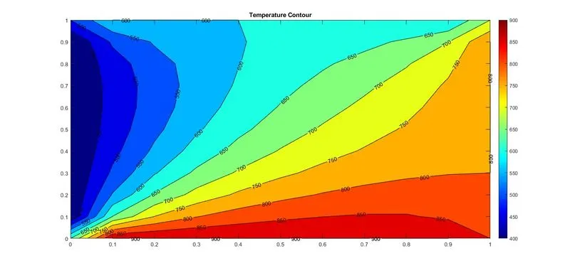
• Temperature contour (in Kelvin) obtained when the problem is solved by using Jacobi - Iterative method

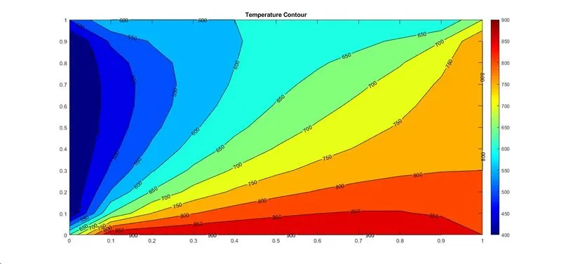
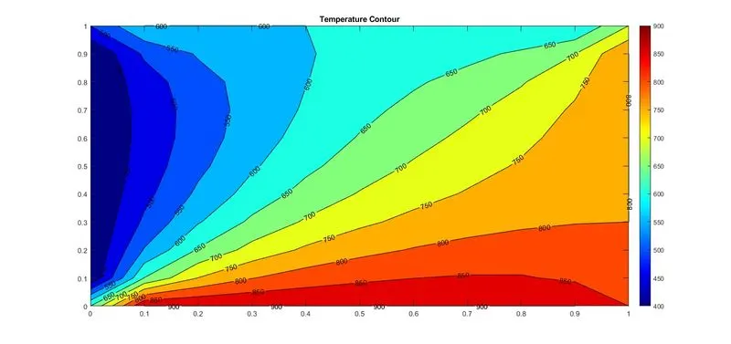
• Temperature contour (in Kelvin) obtained when the problem is solved by using Gauss - Seidel iterative method

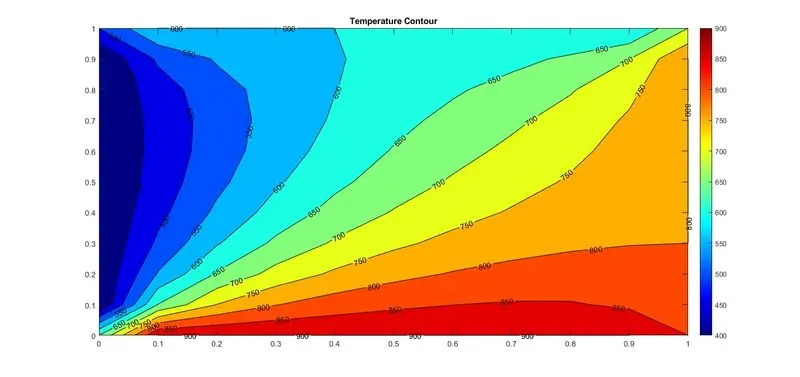
• Temperature contour (in Kelvin) obtained when the problem is solved by using SOR - Iterative method

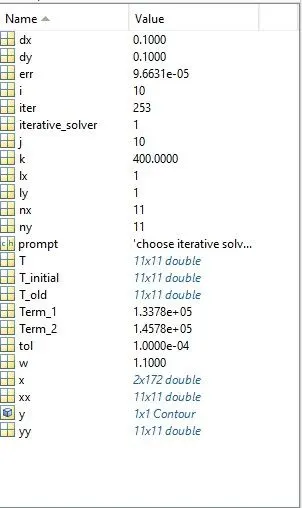
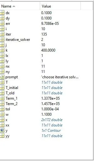
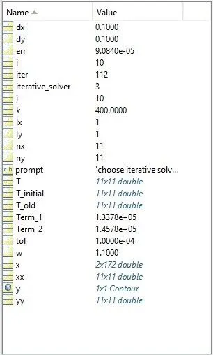
• Comaparison of values obtained from three different cases.

Jacobi Iterative Method Gauss - Seidel Iterative Method SOR - Iterative Method

Unsteady state two-dimensional heat conduction.

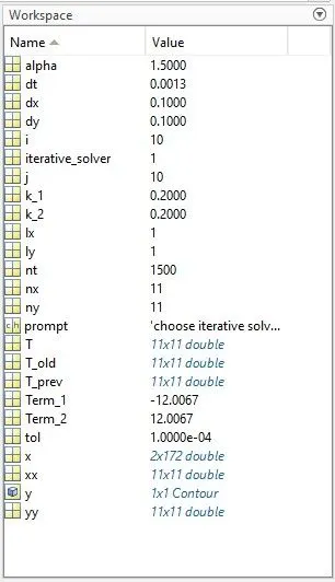
Explicit Method - Iterative solver - 1

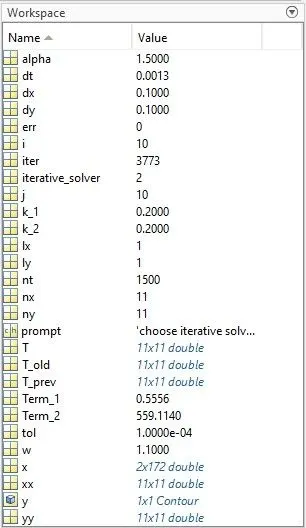
Implicit Method (Jacobi - Iterative Method) - Iterative solver - 2

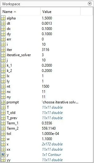
Implicit Method (Gauss - Sediel Iterative Method) - Iterative solver - 3

Implicit Method (SOR - Iterative Method) - Iterative solver - 4

• Temperature contour (in Kelvin) obtained when the problem is solved by using Explicit method

• Temperature contour (in Kelvin) obtained when the problem is solved by using Implicit (Jacobi - Iterative method)

• Temperature contour (in Kelvin) obtained when the problem is solved by using Implicit (Gauss - Seidel iterative method)

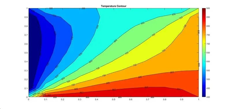
• Temperature contour (in Kelvin) obtained when the problem is solved by using Implicit (SOR - Iterative method)

• Comaparison of values obtained from three different cases.

Explicit Method Implicit - Jacobi Iterative Method Implicit - Gauss - Seidel Iterative Method

Implicit - SOR - Iterative Method

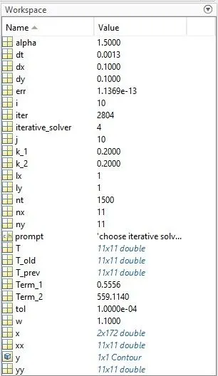
Two -dimensional heat conduction with steady and unsteady case has solved and temperature contours and results are attached above. From the solution it is observed that the iterative solver SOR has fewer number of iteration as compared to other iterative solver. But in the case of SOR the value of relaxation factor plays a vital role, if the value is <1 then under relaxation and if it is >1 over relaxation take place. So to get a convergent solution in case of SOR it is necessary to take a proper value of w. For the case of jacobi solver the number of iteration required for the convergence is very large it is becasue jacobi method use the older value of temperatures to find the new value, where as in Gauss seidel and SOR method the most updated values of temperatures are used for evaluation.

It is also observed that explicit method is easy to solve and it requires less compuational memory as compared to implicit solver. But the explicit method is conditionally stable, that is the stability of explicit method is govern by CFL criteria. But in the case of implicit method there is no such criteria of stability whcih means it is unconditinally stable method.

CONCLUSION:

Two dimensional steady and unsteady state heat conduction problem is solver by using different iterative method and the temperature contours are ploted. A comparison of these results obtained are also carried out during the study and it is cocluded that SOR method with a accurate relaxation factor provides a fast solution as compared to other iterative solver.