Week 5.1 - Mid term project - Solving the steady and unsteady 2D heat conduction problem
Week 5.1 - Mid term project - Solving the steady and unsteady 2D heat conduction problem
Steady State Analysis & Transient State Analysis
Aim : To write a program to Solve the 2D heat conduction equation by using the point iterative techniques.
Key Points :
- Point Iterative techniques.
- Solving Steady state 2D heat conduction equations using Gauss-seidel and Successive over-relaxation techniques implying implicit scheme.
- Solve 2D heat conduction equation for Transient. unsteady state for above 3 methods applying both implicit and explicit schemes.
Point Iterative techniques:
Point iteration method in numerical analysis is used to find an approximate solution to algebraic and transcendental equations. Sometimes, it becomes very tedious to find solutions to cubic, bi-quadratic and transcendental equations; then, we can apply specific numerical methods to find the solution; one among those methods is the fixed point iteration method.
The fixed point iteration method uses the concept of a fixed point in a repeated manner to compute the solution of the given equation. A fixed point is a point in the domain of a function g such that g(x) = x. In the fixed point iteration method, the given function is algebraically converted in the form of g(x) = x.
Suppose we have an equation f(x) = 0, for which we have to find the solution. The equation can be expressed as x = g(x). Choose g(x) such that |g’(x)| < 1 at x = xo where xo,is some initial guess called fixed point iterative scheme. Then the iterative method is applied by successive approximations given by xn = g(xn – 1), that is, x1 = g(xo), x2 = g(x1) and so on.
Explicit and Implicit Methods:
Explicit Method:
The explicit method allows solving problems element by element. Compared with the implicit method, it does not require the general matrix, since the velocity and displacement nodes can be counted directly, using the central difference integration scheme. However, the time step is limited by the size of the numerical stability. Accordingly, this method is considered conditionally stable, because if the time step is too large, there will be a significant numerical error. In this method, there is no requirement for balance, so it is suitable for highly dynamic analysis, such as high-velocity impact.
Implicit Method:
In the implicit method, general equilibrium is achieved by iteration at first, followed by evaluation of local element variables. If the balance is not achieved, this method becomes expensive for calculation, since the matrix coefficients should recalculate with different time steps. The implicit method is unconditionally stable, allowing the use of larger increment time steps. It is suitable for problems that tend to be highly linear, static, and quasi-static.
Governing Equation :
2D heat conduction equation
`(∂T)/(∂t)+α((∂^2 T)/(∂x^2 )+(∂^2 T)/(∂y^2 ))=O`
Where, `alpha =` Thermal diffusivity
We are considering 2 stages of heat conduction i.e.
Steady state and unsteady or transient state.
Steady State Equation Form :
Steady-state conduction is the form of conduction that happens when the temperature difference driving the conduction is constant, so that after an equilibration time, the spatial distribution of temperatures in the conducting object does not change any further. In steady-state conduction, the amount of heat entering any region of an object is equal to the amount of heat coming out (if this were not so, the temperature would be rising or falling, as thermal energy was tapped or trapped in a region).
The Steady State form of the 2-D Heat Conduction Equation is given by,
((∂^2 T)/(∂x^2 )+(∂^2 T)/(∂y^2 ))=O
We will convert above equation into discrete form using following nomenclature.
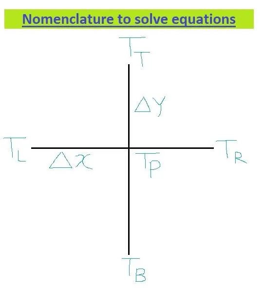
Where,
`T_P=T_(i,j)`
Top Boundary `T_T=T_(i, j+1)`
Bottom Boundary `T_B=T_(i, j-1)`
Left Boundary `T_L=T_(i-1, j)`
Right Boundary `T_R=T_(i+1, j)`
`k=2.((Δx^2+Δy^2)/(Δx^2.Δy^2 ))`
Now putting these values in Steady state equation,
`T_P=1/k ((T_L+T_R)/(Δx^2 ))+1/k ((T_T+T_B)/(Δy^2 ))`
For simplifying calculations, we will call
`Term1=1/k ((T_L+T_R)/(Δx^2 ))` And `Term2= 1/k ((T_T+T_B)/(Δy^2 ))`
We are going to be solving the above forms of equations with the help of 3 iterative techniques. They are,
A. Jacobi Method :
Jacobi method is an iterative algorithm for determining the solutions of a strictly diagonally dominant system of linear equations. Each diagonal element is solved and an approximate value is plugged in. The process is then iterated until it converges.
Each iteration is done using a set of previous values, even if new values are available in the middle of an iteration.Like when you are solving for n+1 iteration and for i th node you will use values of previous(n) iteration even if you have the updated values of the nodes in current iteration.so this method is called method of simultaneous displacements.
The 2D steady state heat conduction equation for this method is,
`T_(i,j)^(n+1)=1/k ((T_(i-1,j)^n+T_(i+1,j)^n)/(Δx^2 )+(T_(i,j-1)^n+T_(i,j+1)^n)/(Δy^2 ))`
B. Gauss-seidel Method :
In Gauss-Seidel, as soon as we find a new value in the current iteration we will use it for finding other values in the current iteration. Like when you are solving for n+1 iteration and for i th node you will use all the available values upto i-1 node of current iteration(n+1) and use i+1 node values and above values of previous iteration(n).SO we get more converged values.so this method is called method of spontaneous displacements.
The 2D steady state heat conduction equation for this method is ,
`T_(i,j)^(n+1) = 1/k ((T(i-1,j)^(n+1)+T_(i+1,j)^n)/(Δx^2 )+(T_(i,j-1)^(n+1)+T_(i,j+1)^n)/(Δy^2 ))`
C. Successive over-relaxation :
It is a variant of the Gauss-Seidel method for solving a linear system of equations, resulting in faster convergence. You can also use jacobi method .Here an extra term called relaxation factor (alpha)is multiplied to gauss seidel generated term to scale the convergence rate and solve the equation faster. To calculate new value we take old value and take a parameter omega and take rate of change.
For scaling Gauss-Seidel method, where Tgs is the result of Gauss-Seidel method.
`T_(i,j)^(n+1)=(1-ω) T_(i,j)^n+ω⋅T_(g_s )`
Where, `omega =`relaxation factor or SOR factor,
when `omega = 0` we get new value is equal to old value which gives wrong result.
`ω<1` Under relaxation
`ω>1` Over relaxation
when omega goes from 0 to 1 we are switching from no update to an update using gauss siedal or jacobi method.
when Omega <1 ,The value we give is called under relaxation factor. This is used when the solution given by gauss siedel is over relaxed we give omega value less than 1 to get the converged solution.
when Omega >1 then we are taking the update from gauss siedal method and scaling up the convergence rate. The value we give is called over relaxation factor.
MATLAB CODE:
Programming Language: MATLAB
Steady State Equations
%Program to solve the 2D Heat Conduction at steady state using Implicit techniques:
clear
close
clc

%% Inputs
%intial Conditions
L=1; % Domain Length
% Domain Defination - No. of nodes
nx=10;
ny=10;

% Given Boundary inputs
T=300*ones(nx,ny); % Temperature Matrix
T(1,:) = 900;   % Bottom Boundary
T(end,:) = 600; % Top Boundary
T(:,1) = 400;   % Left Boundary
T(:,end) = 800; % Right Boundary

%defining space domain
x = linspace(0,L,nx);
y = linspace(0,L,ny);
% grid size
dx = x(2)-x(1);
dy = y(2)-y(1);

% Finding Edges of square domain
T(1,1)=(T(1,2)+T(2,1))/2;
T(1,nx)=(T(1,nx-1)+T(2,nx))/2;
T(ny,1)=(T(ny-1,1)+T(ny,2))/2;
T(ny,nx)=(T(ny,nx-1)+T(ny-1,nx))/2;
Told=T;

error = 100;
tolerance=1e-4; % absolute error criteria
k=2*(dx^2+dy^2)/(dx^2*dy^2);
omega=1.9;   % SOR factor

%% Solver
solver=input('Enter the solver method number: \n Jacobi=1 \n Gauss Seidel=2 \n SOR=3 \n Successive Type: ');
 if solver == 1
%% Jacobi

   tic
   jacobi_iter=1;

        while (error>tolerance) % convergence loop
            for i= 2:(nx-1) % Iteration loop
                for j= 2:(ny-1)

                % calculate the temprature at each grid point
                 Term1=((Told(i-1,j)+Told(i+1,j))/(k*dx^2));
                 Term2=((Told(i,j-1)+Told(i,j+1))/(k*dy^2));
                 T(i,j)= Term1+Term2;
                end
            end
            error = max(max(abs(Told-T)));
            Told = T; % Updating value
            jacobi_iter = jacobi_iter+1;
            timecounter_j=toc;
        end
        %Plot
        figure(1)
        colormap(jet)
        P = contourf(x,y,T,'ShowText','on');
        clabel(P)
        xlabel('xx');
        ylabel('yy');
   title(sprintf('2d Steady State Heat Conduction  \n Method:Jacobi \n No of iterations=%d \n Time:%f s',jacobi_iter,timecounter_j))
  end

    %% Gauss Seidel
   if solver == 2
   tic
   gs_iter=1;
   while (error>tolerance)
        for j=2:ny-1
            for i=2:nx-1
                Term1=((T(i-1,j)+Told(i+1,j))/(k*dx^2));
                Term2=((T(i,j-1)+Told(i,j+1))/(k*dy^2));
                T(i,j)=Term1+Term2;
            end
        end
        error=max(max(abs(Told-T)));
        Told=T;
        gs_iter = gs_iter+1;
        timecounter_1=toc;
    end
    figure(2)
    colormap(jet)
    G = contourf(x,y,T,'ShowText','on');
    clabel(G)
    xlabel('xx');
    ylabel('yy');
title(sprintf('2d Steady State Heat Conduction  \n Method:Gauss Seidel \n No of iterations=%d \n Time:%f s',gs_iter,timecounter_1))
   end


%% Successive
if solver == 3
   tic
   sor_iter=1;
    while (error>tolerance)
        for j=2:ny-1
            for i=2:nx-1
                 Term1=((T(i-1,j)+Told(i+1,j))/(k*dx^2));
                 Term2=((T(i,j-1)+Told(i,j+1))/(k*dy^2));
                 T(i,j)=(Told(i,j)*(1-omega))+(omega*(Term1+Term2));
            end
        end
        error=max(max(abs(Told-T)));
        Told=T;
        sor_iter=sor_iter+1;
        timecounter_2=toc;
 end
      figure(3)
      colormap(jet)
      S = contourf(x,y,T,'ShowText','on');
      clabel(S)
      xlabel('xx');
      ylabel('yy');
    title(sprintf('2d Steady State Heat Conduction  \n Method:SOR \n No of iterations=%d \n Time:%f s',sor_iter,timecounter_2))
    end
Output for Steady State Heat Conduction :
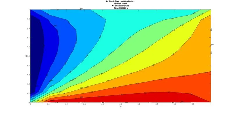
A. Steady state equation using Jacobi Method:
No. of Iteration : 208 Time Required: 0.00958 Sec.
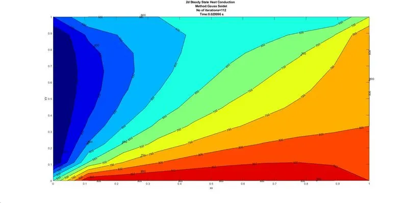
B. Gauss-Seidel Method:
No. of Iteration : 112
Time Required: 0.029996 Sec.
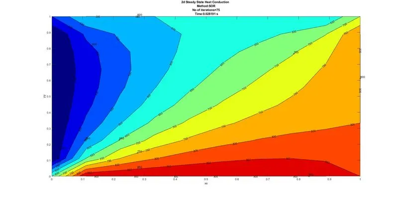
C. Successive over-relaxation(SOR) :
No. of Iteration : 75
Time Required: 0.028191 Sec.
Transient or Unsteady State:
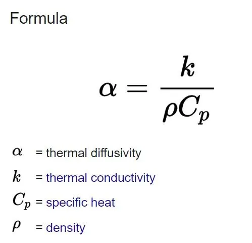
For transient state we have to introduce thermal diffusivity.
In heat transfer analysis, thermal diffusivity is the rate of temperature spread through a material. It is defined as the thermal conductivity divided by density and specific heat capacity at constant pressure. It is denoted by alpha (`alpha`)
Transient Equation Form :
During any period in which temperatures changes in time at any place within an object, the mode of thermal energy flow is termed transient conduction. Another term is "non-steady-state" conduction, referring to the time-dependence of temperature fields in an object.
The Transient form of the 2-D Heat Conduction Equation is given by,
`(∂T)/(∂t)-α((∂^2 T)/(∂x^2 )+(∂^2 T)/(∂y^2 ))=O`
Now we know that
`(∂T)/(∂t)=(T_((i,j))^(n+1)-T_((i,j))^n)/(Δt)`
`(∂^2 T)/(∂x^2 )= (T_((i+1,j))^n-2T_((i,j))^n+T_((i-1,j))^n)/(Δx^2 )`
`(∂^2 T)/(∂y^2 )= (T_((i,j+1))^n-2T_((i,j))^n+T_((i,j-1))^n)/(Δy^2 )`
Substituting these discretized values in the Transient Equation and simplifying, we get,
`T_((i,j))^(n+1)=T_((i,j))^n+((α.Δt)/(Δx^2.Δy^2 )) ((T_((i+1,j))^n-2T_((i,j))^n+T_((i-1,j))^n)+(T_((i,j+1))^n-2T_((i,j))^n+T_((i,j-1))^n))`
Consider following terms to simplification of Unsteady equation
`k_1=α⋅Δt/(Δx^2 )` and `k_2=α⋅Δt/(Δy^2 )`
`T_((i,j))^(n+1)=T_((i,j))^n+k1 [T_((i+1,j))^n-2T_((i,j))^n+T_((i-1,j))^n]+k2[T_((i,j+1))^n-2T_((i,j))^n+T_((i,j-1))^n]`
Explicit Vs Implicit Techniques
|
Explicit Techniques |
Implicit Techniques |
|
Function solved with help of dependent variable. |
Function cannot solved with help of dependent variable only. So in this case, we required iteration methods. |
|
It calculates the state of a system at a later time from the state at the current time. |
Implicit method finds a solution by solving an equation involving both the current state of the system and the later state. |
|
Explicit methods require small time steps to keep the error in the result bounded. |
This method considers simultaneous equations and uses guess values as the initial values to find the approximated values. If the guess values are closer to the desired value the computation time will be less. |
|
With the decrease in time step the number of computations increases and hence the computational time required to converge is less and the accuracy of the solution is high. |
The computational time required for the solution to converge is high and the accuracy of the solution is less. There is no stability criteria requirement so more significant time steps can be used. It requires an extra computation since the matrix coefficients should recalculate with different time steps. |
|
Therefore, It is also called as Direct Solver Technique. |
Implicit is also known as Iteration Solver Technique. |
MATLAB CODE:
Unsteady State Equation by Explicit Techniques
%Program to solve the 2D Heat Conduction at Transient state using Explicit techniques:
clear
close
clc

%% Inputs
%intial Conditions
L=1; % Domain Length
% Domain Defination - No. of nodes
nx=10;
ny=10;

% Given Boundary inputs
T=300*ones(nx,ny); % Temperature Matrix
T(1,:) = 900;   % Bottom Boundary
T(end,:) = 600; % Top Boundary
T(:,1) = 400;   % Left Boundary
T(:,end) = 800; % Right Boundary

%defining space domain
x = linspace(0,L,nx);
y = linspace(0,L,ny);
% grid size
dx = x(2)-x(1);
dy = y(2)-y(1);

% Finding Edges of square domain
T(1,1)=(T(1,2)+T(2,1))/2;
T(1,nx)=(T(1,nx-1)+T(2,nx))/2;
T(ny,1)=(T(ny-1,1)+T(ny,2))/2;
T(ny,nx)=(T(ny,nx-1)+T(ny-1,nx))/2;
Told=T;

% Inputs for time variables

dt = 0.001;
nt = 1400; %nt = dt/t

e = 100; % Error
tolerance=1e-4; % absolute error criteria

alpha = 1.4; %Thermal diffusivity

K1 = alpha*(dt/dx^2); %cfl value for x
K2 = alpha*(dt/dy^2); %cfl value for y

% CFL Number calculation and adaptive Time-step control:
CFL_Number = K1+K2

%% Explicit Method
   tic
   for m = 1:nt %Time loop
       for i= 2:(nx-1) % Iteration loop
            for j= 2:(ny-1)

            % calculate the temprature at each grid point
            H=(Told(i-1,j)+Told(i+1,j)-(2*Told(i,j))); % Temp values in X-direction
            V=(Told(i,j-1)+Told(i,j+1)-(2*Told(i,j))); % Temp values in Y-direction
            % Point-wise temp
            T(i,j)= (Told(i,j)+(H*K1)+(V*K2));
            end
        end
        Told = T; % Updating value
   end
   timecounter_Explicit=toc;
   %Plot
    figure(1)
    colormap(jet)
    P = contourf(x,y,T,'ShowText','on');
    clabel(P)
    xlabel('xx');
    ylabel('yy');
    title(sprintf('2d Transient State Heat Conduction \n Method: Explicit \n Time: %f s \n CFL Number: %f \n',timecounter_Explicit,CFL_Number))
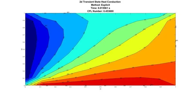
Output for Unsteady State Heat Conduction by Explicit Techniques :
Time Required: 0.015561 Sec.
CFL Number : 0.4536
Transient or Unsteady State equation by Implicit Techniques:
Implicit methods are approaches used in numerical analysis for obtaining numerical approximations to the solutions of time-dependent ordinary and partial differential equations, as is required in computer simulations of physical processes. Implicit methods find a solution by solving an equation involving both the current state of the system (n) and the later one (n+1).
Discretizing the Transient Equation Form by employing Central Difference Scheme for the second order derivative terms, therefore, the discretized terms are as follows.
`(∂T)/(∂t)=(T_((i,j))^(n+1)-T_((i,j))^n)/(Δt)`
`(∂^2 T)/(∂x^2 )= (T_((i+1,j))^(n+1)-2T_((i,j))^(n+1)+T_((i-1,j))^(n+1))/(Δx^2 )`
`(∂^2 T)/(∂y^2 )= (T_((i,j+1))^(n+1)-2T_((i,j))^(n+1)+T_((i,j-1))^(n+1))/(Δy^2 )`
Substituting these discretized values in the Transient Equation and simplifying, we get,
`T_((i,j))^(n+1)=T_((ⅈ,j))^n+((α.Δt)/(Δx^2.Δy^2 )) ((T_((ⅈ+1,j))^(n+1)-2T_((ⅈ,j))^(n+1)+T_((ⅈ-1,j))^(n+1))+(T_((ⅈ,j+1))^(n+1)-2T_((ⅈ,j))^(n+1)+T_((ⅈ,j-1))^(n+1)))`
Consider following terms to simplification of Unsteady equation
`k_1=α⋅(Δt)/(Δx^2 )` And `k_2=α⋅(Δt)/(Δy^2 )`
`T_((i,j))^(n+1)=T_((i,j))^n+k1 [T_((i+1,j))^(n+1)-2T_((ⅈ,j))^(n+1)+T_((ⅈ-1,j))^n]+k2[T_((ⅈ,j+1))^(n+1)-2T_((i,j))^(n+1)+T_((i,j-1))^(n+1)]`
Now simplifying above equation, we will get
`T_((i,j))^(n+1)= (1/(1+2k_1+2k_2 ))[T_((ⅈ,j))^n+k1 [T_((ⅈ+1,j))^(n+1)+T_((ⅈ-1,j))^n]+k2[T_((ⅈ,j+1))^(n+1)+T_((ⅈ,j-1))^(n+1)]]`
For simplification, we will split above equation as,
`Term 1 = (1/(1+2k_1+2k_2 ))`
`Term 2 = k1*Term 1`
`Term 3 = k2*Term 1`
Now final equation becomes,
`T_((i,j))^(n+1)= Term1*T_((i,j))^n+Term2*[T_((i+1,j))^(n+1)+T_((i-1,j))^n ]+Term3*[T_((i,j+1))^(n+1)+T_((i,j-1))^(n+1)]`
Now, we will use following 3 methods to get temperature values at each grid point.
A. Jacobi Method :
`T_((i,j))^(n+1)= Term1*T_((i,j))^n+Term2*[T_((i+1,j))^n+T_((i-1,j))^n ]+Term3*[T_((i,j+1))^n+T_((i,j-1))^n]`
B. Gauss- Seidel Method :
`[T_(gs) ]=T_((i,j))^(n+1)= Term1*T_((i,j))^n+Term2*[T_((i+1,j))^(n+1)+T_((i-1,j))^n ]+Term3*[T_((i,j+1))^(n+1)+T_((i,j-1))^(n+1)]`
C. Successive Over-relaxation Method :
`T_((i,j))^(n+1)= (1-ω)*T_((i,j))^n+ω*[T_(gs) ]`
MATLAB CODE:
Unsteady State Equation by Implicit Techniques
%Program to solve the 2D Heat Conduction at Transient state using Implicit techniques:
clear
close
clc

%% Inputs
%intial Conditions
L=1; % Domain Length
% Domain Defination - No. of nodes
nx=10;
ny=10;

% Given Boundary inputs
T=300*ones(nx,ny); % Temperature Matrix
T(1,:) = 900;   % Bottom Boundary
T(end,:) = 600; % Top Boundary
T(:,1) = 400;   % Left Boundary
T(:,end) = 800; % Right Boundary

%defining space domain
x = linspace(0,L,nx);
y = linspace(0,L,ny);
% grid size
dx = x(2)-x(1);
dy = y(2)-y(1);

% Finding Edges of square domain
T(1,1)=(T(1,2)+T(2,1))/2;
T(1,nx)=(T(1,nx-1)+T(2,nx))/2;
T(ny,1)=(T(ny-1,1)+T(ny,2))/2;
T(ny,nx)=(T(ny,nx-1)+T(ny-1,nx))/2;
Told=T;

T_prev_dt = Told;
alpha = 1.4; %Thermal diffusivity
dt = 0.01;
nt = 1400;
e = 100; % Error

tolerance=1e-4; % absolute error criteria

k = 2*(dx^2+dy^2)/(dx^2*dy^2);
K1 = alpha*(dt/dx^2); %cfl value for x
K2 = alpha*(dt/dy^2); %cfl value for y
Term1 = (1+2*K1+2*K2)^-1;
Term2 = K1*Term1;
Term3 = K2*Term1;
omega = 1.2;   % SOR factor

%% Solver
solver=input('Enter the solver method number: \n Jacobi=1 \n Gauss Seidel=2 \n SOR=3 \n Successive Type: ');
if solver == 1
%% Jacobi

   tic
   jacobi_iter=1;
   for m = 1:nt %Time loop
       error = e;
     while (error>tolerance) % convergence loop
       % Iteration loop
        for i= 2:(nx-1)
            for j= 2:(ny-1)

        % calculate the temprature at each grid point
        H=(Told(i-1,j)+Told(i+1,j)); % Temp values in X-direction
        V=(Told(i,j-1)+Told(i,j+1)); % Temp values in Y-direction
        % Point-wise temp
        T(i,j)= (T_prev_dt(i,j)*Term1)+(H*Term2)+(V*Term3);
            end
        end
        error = max(max(abs(Told-T)));
        Told = T; % Updating value
        jacobi_iter = jacobi_iter+1;
     end
     T_prev_dt = T;
   end
   timecounter_j=toc;
   %Plot
    figure(1)
    colormap(jet)
    P = contourf(x,y,T,'ShowText','on');
    clabel(P)
    xlabel('xx');
    ylabel('yy');
    title(sprintf('2d Transient State Heat Conduction  \n Method: Implicit Jacobi \n No of iterations=%d \n Time:%f s',jacobi_iter,timecounter_j))
end

    %% Gauss Seidel
 if solver == 2
   tic
   gs_iter=1;
  for m = 1:nt %Time loop
       error = e;

    while (error>tolerance)
        for j=2:(ny-1)
            for i=2:(nx-1)
                H=(T(i-1,j)+Told(i+1,j));
                V=(T(i,j-1)+Told(i,j+1));
                T(i,j)=(T_prev_dt(i,j)*Term1)+(H*Term2)+(V*Term3);
            end
        end
        error=max(max(abs(Told-T)));
        Told=T;
        gs_iter = gs_iter+1;
    end
   T_prev_dt = T;
  end
        timecounter_G=toc;
    %Plot
    figure(2)
    colormap(jet)
    G = contourf(x,y,T,'ShowText','on');
    clabel(G)
    xlabel('xx');
    ylabel('yy');
title(sprintf('2d Transient State Heat Conduction  \n Method: Implicit Gauss Seidel \n No of iterations=%d \n Time:%f s',gs_iter,timecounter_G))
 end


%% Successive
if solver == 3
   tic
   sor_iter=1;
  for m = 1:nt %Time loop
       error = e;
    while (error>tolerance)
        for j=2:(ny-1)
            for i=2:(nx-1)
                 H = (T(i-1,j)+Told(i+1,j));
                 V = (T(i,j-1)+Told(i,j+1));
                 Tgs = (T_prev_dt(i,j)*Term1)+(H*Term2)+(V*Term3);
                 T(i,j)=(Told(i,j)*(1-omega))+(omega*Tgs);
            end
        end
        error=max(max(abs(Told-T)));
        Told=T;
        sor_iter=sor_iter+1;
    end
    T_prev_dt = T;
  end
    timecounter_SOR=toc;
     % Plot
      figure(3)
      colormap(jet)
      S = contourf(x,y,T,'ShowText','on');
      clabel(S)
      xlabel('xx');
      ylabel('yy');
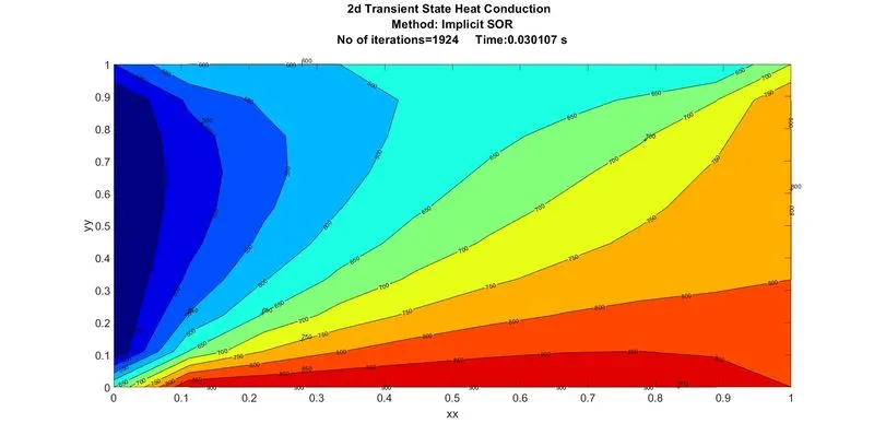
    title(sprintf('2d Transient State Heat Conduction  \n Method: Implicit SOR \n No of iterations=%d     Time:%f s \n  ',sor_iter,timecounter_SOR))
end
Output for Unsteady State Heat Conduction by Implicit Techniques :
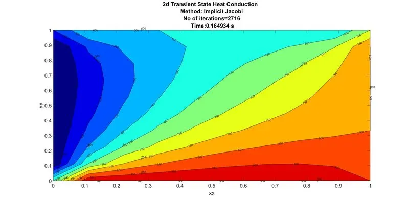
A. Jacobi Method:
No. of Iteration : 2716
Time Required: 0.164934 Sec.
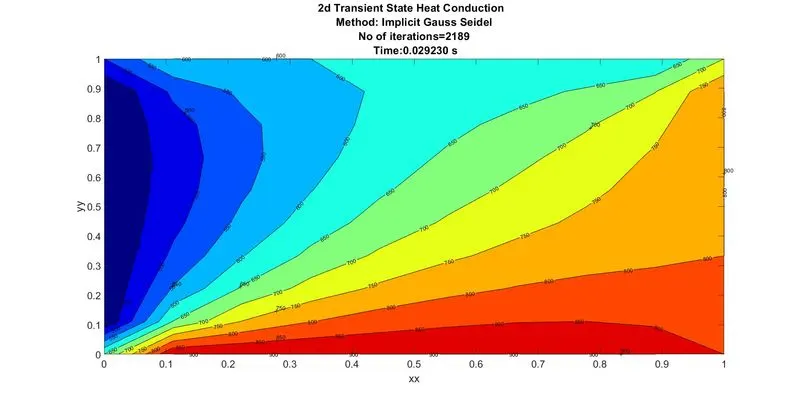
B. Gauss-Seidel Method:
No. of Iteration : 2189
Time Required: 0.029230 Sec.
C. SOR Method:
No. of Iteration : 2716 Time Required: 0.164934 Sec.
Numeric Diffusion :
- Numerical diffusion appears in multi-dimensional flows when the differencing scheme fails to account for the true direction of the flow.
- It is Error in discretization, formulation of the finite difference equations, or just machine precision can all cause an increase in (thermal/momentum) diffusivity of the material being simulated, causing the results to be (sometimes wildly) inaccurate.
- Numerical or false diffusion is the phenomenon of inserting errors in the calculations that compromise the accuracy of the computational solution.
- A numerical scheme must satisfy necessary criteria for the successful solution of the convection-diffusion formulations. The common practice of approximating the diffusion terms via the central-difference approximation is satisfactory. Attention is directed to the convection terms since these approximations induce false diffusion. The equations of all the conservation equations in this study are discretized by the finite volume method.
- Numerical diffusion is a significant source of error in numerical solution of conservation equations and can be separated into two components namely cross-stream and streamwise numerical diffusion. The former occurs when gradients in a convected quantity exist perpendicular to the flow and the direction of the flow is oblique to the grid lines, i.e. due to the multi-dimensional nature of the flow.
- This diffusion is dependent on the factor called as Courant number
- This CFL number determines the level of instability in the particular problem.
- It must be below 1 and should ideally be below 0.7. If the Courant number exceeds 1, the time step is too large to see the particle in one cell, it “skips” the cell and cause instability.
Conclusion :
- We have solved 2D heat conduction equation for both Steady and Transiente. Unsteady state by implementing Implicit Technique. For iteration purpose we used 3 methods i.e. Jacobi, Gauss-Seidel, Successive Over Relaxation (SOR).
- For both Steady and Unsteady state we found out that SOR method required less number of iteration and less time to give result compared to Jacobi and Gauss-Seidel. So we can arrange order with respective number of iteration and time required to get result as follows,
- SOR < Gauss-Seidel < Jacobi.
- We also applied Explicit technique to Unsteady state heat conduction and we observed that if we keep Explicit method required less time compared to Implicit techniques but stability of result depend on CFL number used in Explicit techniques. To get ideal result using explicit method we must kept CFL number below 0.45 and above 0.02
- So, we can conclude that Successive Over Relaxation (SOR) method with Implicit technique is most efficient method to solve 2D Heat conduction equation for both Steady and transient state.
Reference:
- https://home.iitk.ac.in/~psraj/mth101/lecture_notes/lecture8.pdf
- https://www.maa.org/press/periodicals/loci/joma/iterative-methods-for-solving-iaxi-ibi-the-sor-method
- https://ijmttjournal.org/2018/Volume-56/number-4/IJMTT-V56P531.pdf
- https://il.water.usgs.gov/proj/feq/feqdoc/chap2html/chap2_4.html
- https://www.intechopen.com/chapters/60679