Week 5.1 - Mid term project - Solving the steady and unsteady 2D heat conduction problem
Program-1: Steady state (Explicit method)
% Steady state problem (Explicit method)


clear all;
close all;
clc;
%No. of nodes in x & y
nx = 10;
ny = 10;

%Variation of T in x & y

T = ones(nx,ny);

T(2:end-1,1) = 400;
T(2:end-1,end) = 800;
T(1,2:end-1) = 600;
T(end,2:end-1) =  900;
T(1,1) = (600+400)/2;
T(1,end) = (600+800)/2;
T(end,1) = (400+900)/2;
T(end,end) =  (800+900)/2;


%length of domain in x & y
lx = 1;
ly = 1;

% step size in x & y
dx = lx/(nx-1);
dy = ly/(ny-1);
x = 0:dx:lx;
y = 0:dy:ly;


T_old = T;
T_initial = T_old;
error = 10;
tol = 1e-4;
iteration = 0;
term_1 = 2*(dx^2 + dy^2)/(dx^2*dy^2);

iteration_method = input('What will be the iteration method . 1-Jacobi, 2-Gauss Siedel, 3- SOR');
if iteration_method == 1      %Jacobi
    tic;
    while(error > tol)
        iteration = iteration +1;
        disp(iteration)
        for i = 2:nx-1
            for j = 2:ny-1
                term_2 = (T_old(i-1,j)+T_old(i+1,j))/(term_1*(dx^2));
                term_3 = (T_old(i,j-1)+T_old(i,j+1))/(term_1*(dy^2));
                T(i,j) = term_2 + term_3;

            end
        end
        error=max(max(abs(T_old-T)));
        T_old = T;
    end
    time = toc;
end

if iteration_method == 2      %Gauss siedel method
    tic;
    while(error > tol)
        iteration = iteration +1;
        disp(iteration)
        for i = 2:nx-1
            for j = 2:ny-1
                term_2 = (T(i-1,j)+T_old(i+1,j))/(term_1*(dx^2));
                term_3 = (T(i,j-1)+T_old(i,j+1))/(term_1*(dy^2));
                T(i,j) = term_2 + term_3;

            end
        end
        error=max(max(abs(T_old-T)));
        T_old = T;
    end
    time = toc;
end

if iteration_method == 3      %SOR
    omega = 1.6;
    tic;
    while(error > tol)
        iteration = iteration +1;
        disp(iteration)
        for i = 2:nx-1
            for j = 2:ny-1
                term_2 = (T(i-1,j)+T_old(i+1,j))/(term_1*(dx^2));
                term_3 = (T(i,j-1)+T_old(i,j+1))/(term_1*(dy^2));
                T(i,j) = term_2 + term_3;
                T(i,j) = T_old(i,j)*(1-omega) + omega*(T(i,j));

            end
        end
        error=max(max(abs(T_old-T)));
        T_old = T;
    end
    time = toc;
end


    figure(1)
    [a,b] = contourf(x,y,T);
    clabel(a,b)
    colormap(jet)
    colorbar
    set(gca,'ydir','reverse')
    pause (0.03)
    xlabel('x')
    ylabel('y')
    title({'Steady state 2D conduction';['Iteration Method = ',num2str(iteration_method)];['No. of iterations = ',num2str(iteration)];['Simulation time = ',num2str(time),' s']})
    grid on
Program-2: Transient state 2D heat conduction ( Explicit method)
% Unsteady state problem (Explicit method)


clear all;
close all;
clc;
%No. of nodes in x & y
nx = 50;
ny = 50;

%Variation of T in x & y

T = ones(nx,ny);

T(2:end-1,1) = 400;
T(2:end-1,end) = 800;
T(1,2:end-1) = 600;
T(end,2:end-1) =  900;
T(1,1) = (600+400)/2;
T(1,end) = (600+800)/2;
T(end,1) = (400+900)/2;
T(end,end) =  (800+900)/2;

%Time duration
dt = 0.1;
t = 50;
nt = t/dt;

%length of domain in x & y
lx = 1;
ly = 1;

% step size in x & y
dx = lx/(nx-1);
dy = ly/(ny-1);
x = 0:dx:lx;
y = 0:dy:ly;


alpha = 1.4;
T_old = T;
T_initial = T_old;
error = 10;
tol = 1e-4;
iteration = 0;
k1 = alpha*dt/dx^2;
k2 = alpha*dt/dy^2;
term_1 = 1/(1+2*k1+2*k2);

tic;
for l =1:nt
    while(error>tol)

    for i = 2:nx-1
        for j = 2:ny-1
            iteration = iteration +1;
            disp(iteration)
            term_2 = k1*term_1;
            term_3 = k2*term_1;

            T(i,j) = term_1*T_old(i,j)+(term_2*(T_old(i-1,j)+T_old(i+1,j)))+(term_3*(T_old(i,j-1)+T_old(i,j+1)));


        end
        error = max(max(abs(error-tol)));

        T_old = T;
    end

    end
end
time = toc;

figure(1)
[a,b] = contourf(x,y,T);
clabel(a,b)
colormap(jet)
colorbar
set(gca,'ydir','reverse')
pause (0.03)
xlabel('x')
ylabel('y')
title({'Unsteady state 2D conduction, Explicit method';['No. of iterations = ',num2str(iteration)];['Simulation time = ',num2str(time),' s'];['Time =', num2str(t)]})
grid on
Program-3: Transient state 2D heat conduction (Implicit method)
% Unsteady state problem (Implicit method)


clear all;
close all;
clc;
%No. of nodes in x & y
nx = 50;
ny = 50;

%Variation of T in x & y

T = ones(nx,ny);

T(2:end-1,1) = 400;
T(2:end-1,end) = 800;
T(1,2:end-1) = 600;
T(end,2:end-1) =  900;
T(1,1) = (600+400)/2;
T(1,end) = (600+800)/2;
T(end,1) = (400+900)/2;
T(end,end) =  (800+900)/2;

%Time duration
dt = 13;
t = 1000;
nt = t/dt;

%length of domain in x & y
lx = 1;
ly = 1;

% step size in x & y
dx = lx/(nx-1);
dy = ly/(ny-1);
x = 0:dx:lx;
y = 0:dy:ly;


T_old = T;
T_prev = T;

tol = 1e-4;
error = 20;
iteration = 0;

alpha = 0.009;
k1 = alpha*dt/dx^2;
k2 = alpha*dt/dy^2;
CFL = k1+k2;
term_1 = 1/(1+2*k1+2*k2);


iteration_method = input('What will be the iteration method . 1-Jacobi, 2-Gauss Siedel, 3- SOR');

tic
if iteration_method == 1      %Jacobi

    for m =1:nt   % Time loop
        while(error > tol)
            iteration = iteration +1;
            for i = 2:nx-1      % space loop
                for j = 2:ny-1
                    term_2 = k1*term_1;
                    term_3 = k2*term_1;
                    T(i,j) = term_1*T_prev(i,j)+(term_2*(T_old(i-1,j)+T_old(i+1,j)))+(term_3*(T_old(i,j-1)+T_old(i,j+1)));
                end
            end
            error = max(max(abs(error-tol)));     %error term
            T_old = T;
            iteration = iteration +1;
        end
        T_prev = T;
    end

elseif iteration_method == 2      %Gauss Siedel
    for m =1:nt   % Time loop
        while(error > tol)
            iteration = iteration+1;
            for i = 2:nx-1      % space loop
                for j = 2:ny-1
                    term_2 = k1*term_1;
                    term_3 = k2*term_1;
                    T(i,j) = term_1*T_prev(i,j)+(term_2*(T(i-1,j)+T_old(i+1,j)))+(term_3*(T(i,j-1)+T_old(i,j+1)));
                end
            end
            error = max(max(abs(error-tol)));     %error term
            T_old = T;
            iteration = iteration +1;
        end
        T_prev = T;
    end

elseif iteration_method == 3      %SOR
    omega = 1.6;
        for m =1:nt   % Time loop
            while(error > tol)
                for i = 2:nx-1      % space loop
                    for j = 2:ny-1
                        term_2 = k1*term_1;
                        term_3 = k2*term_1;
                        T(i,j) = term_1*T_prev(i,j)+(term_2*(T(i-1,j)+T_old(i+1,j)))+(term_3*(T(i,j-1)+T_old(i,j+1)));
                        T(i,j) = T_old(i,j)*(1-omega)+omega*T(i,j);
                    end
                end
                error = max(max(abs(error-tol)));     %error term
                T_old = T;
                iteration = iteration +1;
            end
            T_prev = T;
        end
end
time = toc;        % simulation time

figure(1)
[a,b] = contourf(x,y,T);
clabel(a,b)
colormap(jet)
colorbar
set(gca,'ydir','reverse')
pause (0.03)
xlabel('x')
ylabel('y')
title({'Unsteady state 2D conduction, Implicit method';['No. of iterations = ',num2str(iteration)];['Simulation time = ',num2str(time),' s'];['Time =', num2str(t)]})
grid on
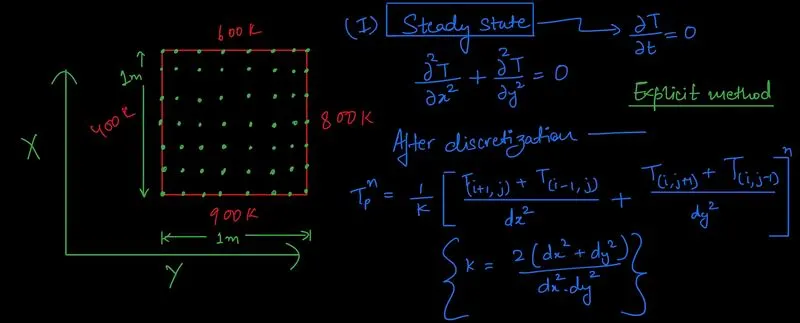
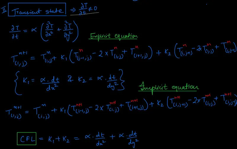
The images below show the governing equations (Steady state & Transient state) and the problem description
% Boundary conditions,
Considering left wall temp = 400K, right wall temp = 800K, Top wall temp = 600K , Bottom wall temp = 900K. Also taking the average of the adjacent wall temps at the corners.
Results: Steady State (1: Jacobi, 2: Gauss Siedel, 3: SOR)
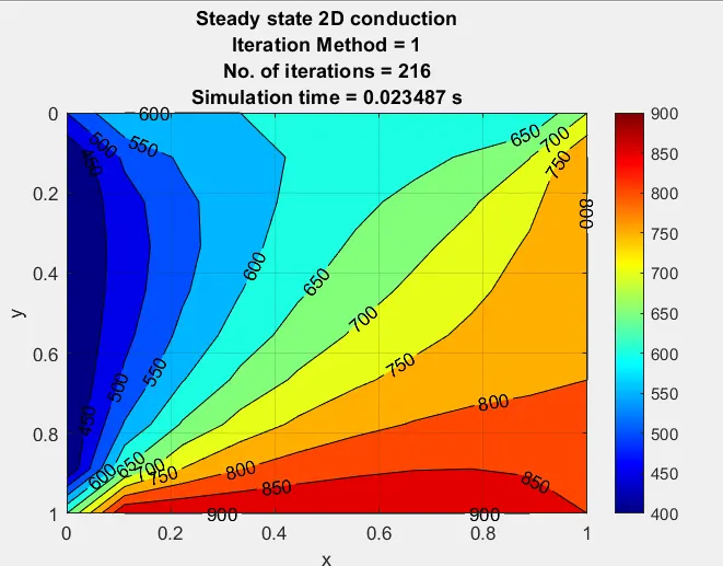
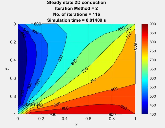
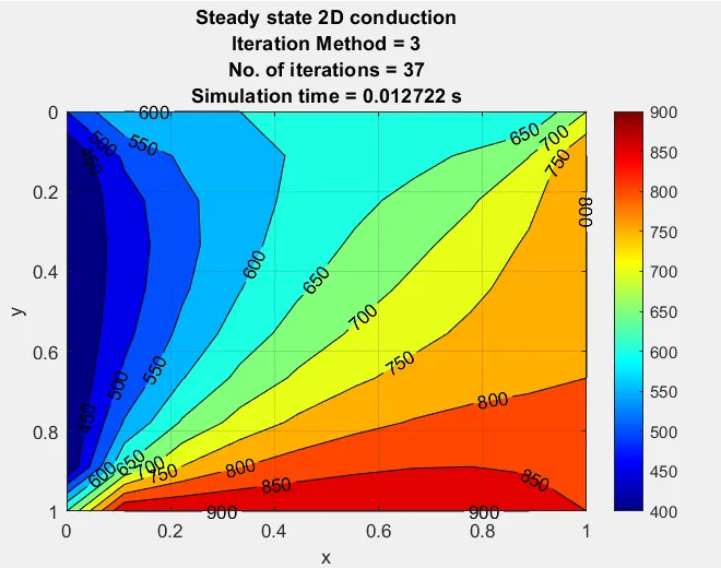
In these graphs, we can see that No. of iterations by Jacobi > Gauss Siedel > SOR
Results: Transient State (Explicit form)
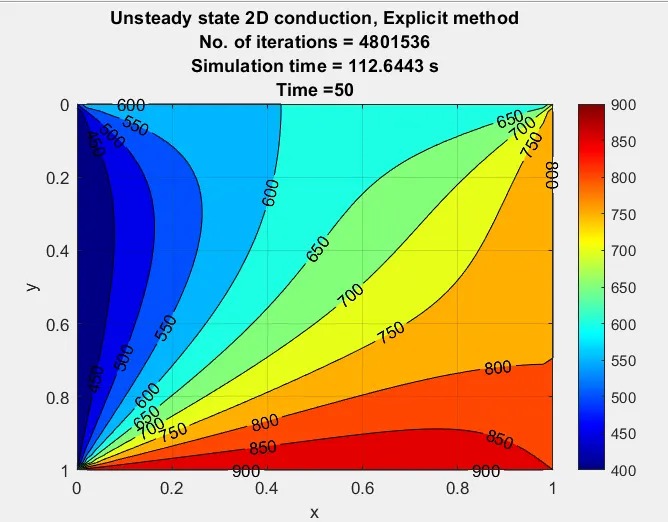
In the Explicit method basically, all the terms on the RHS are at computed at 'nth' time step.
Results: Transient state (Implicit form) (1: Jacobi, 2: Gauss Siedel, 3: SOR)
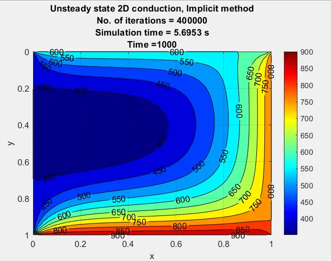
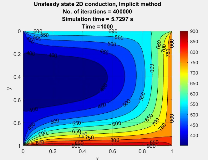
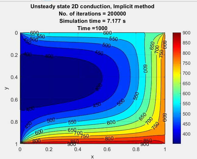
It took half iterations to solve by SOR as compared to Jacobi.