Genetic Algorithm using MATLAB

Week 4 - Genetic Algorithm in MATLAB

AIM: To understand the concept of genetic algorithm and optimize stalagmite function and ways to optimise it.

OBJECTIVES:

(1) Write a code in MATLAB to optimise the stalagmite function and find the global maxima of the function.

(2) Explain the concept of the genetic algorithm and its syntax.

(3) Plot graphs for all 3 studies and for F maximum vs no. of iterations.

BRIEF:

A genetic algorithm (GA) is a method for solving both constrained and unconstrained optimization problems based on a natural selection process that mimics biological evolution. The algorithm repeatedly modifies a population of individual solutions. At each step, the genetic algorithm randomly selects individuals from the current population and uses them as parents to produce the children for the next generation. Over successive generations, the population "evolves" toward an optimal solution.

You can apply the genetic algorithm to solve problems that are not well suited for standard optimization algorithms, including problems in which the objective function is discontinuous, nondifferentiable, stochastic, or highly nonlinear. The genetic algorithm can address problems of mixed-integer programming, where some components are restricted to be integer-valued.

The genetic algorithm uses three main types of rules at each step to create the next generation from the current population:

Syntax: x = ga(fun,nvars)

Where it finds a local unconstrained minimum, 'x', to the objective function, 'fun' and 'nvars' is the dimension (number of design variables) of 'fun'.

For example:

rng default % For reproducibility
x = ga(@ps_example,2)

Here, the function=ps_example is created and solve the equations which the GA has to solve and pick any random values closes to the accuracy to find the minima of the function and '2' are the number of variables in the equation.

Stalagmite functions:

• A stalagmite is a type of rock formation that rises from the floor of a cave due to the accumulation of material deposited on the floor from ceiling drippings. Stalagmites are typically composed of calcium carbonate but may consist of lava, mud, peat, pitch, sand, sinter and amber.
• It is generally referred to the function with which we are generating values over a stalagmite kind of surface for finding the local and the global maxima of the function.
• In MATLAB, we use 'optimization'. It is the decision-making process to find out the best results under a set of prioritization criteria or constraints.
• To use the optimization procedure, we use GA which is an inbuilt function which helps to find the best results using the random values for the set of inputs provided.

Ways to optimize the stalagmite function:

(1) Setting up the bound limit, so that the GA finds the best results in the given range.

(2) By increasing the population size.

Stalagmite Equations for force calculation:

`fx_1 = [sin(5.1pix)+0.5)]^6`
`fy_1 = [sin(5.1piy)+0.5)]^6`
`fx_2 = exp[-4ln(2)((x-0.0667)^2)/(0.64)]`
`fy_2 = exp[-4ln(2)((y-0.0667)^2)/(0.64)]`
`f = (fx_1*fx_2*fy_1*fy_2)`

CODE LOGIC:

(1) Define the two 1D inputs `x` and `y` into an evenly spaced array containing 150 elements. We utilise the mesh grid command to create an array of `x` and `y` values.

(2) Now we use the for loop to input values of the 2D array in stalagmite function. Here we encounter a problem,i.e. every time the code is executed different values for stalagmite function are obtained. This is overcome by introducing another for loop into the code. We then input these values in the genetic algorithm. For genetic algorithm 'ga' function is used.

(3) Create the function for stalagmite by using the above-mentioned formulae into 4 terms for convenience to calculate the force for both the variables for each value.

(4) To improve our Genetic Algorithm, we undertake three cases to optimise the function so that we can accurately find the global maxima of the function. We need to do this because the GA randomly takes the values and global maxima changes according to that.

Case 1: We evaluate all the possible global maxima for all the iterations using a loop.

Case 2: We set the bound limit on the 'ga' function such as upper bound and lower bound

Case 3: We increase the population size fo more GA iterations.

(5) Create another function 'get_stalagmite' for calculating the values for both the variables for each time the code runs using a 'for-loop' command.

(6) Plot the graph for all the cases to visualise the global maxima of the function. We use 'surfc' command to plot the values of `x`, `y` & `f`. Also, plot the graph for 'F maximum vs no. of iterations' for each case.

(7) To find the time execution of each case, we use 'tic-toc' command to define the study time.

NOTE: The force is displayed is shown by `-f`, as GA finds the minima of the function, so by introducing the negative sign it will invert the values of `f` to get the global maxima of the function.

The output is shown in the results section.

CODE:
(1) The stalagmite function:

% Creating a function for Stalagmite

function [f] = stalagmite(input_vector)
x = input_vector(1);
y = input_vector(2);

f1x = (sin((5.1*pi.*x)+0.5)).^6;
f1y = (sin((5.1*pi.*y)+0.5)).^6;
f2x = exp((-4*log(2)).*(((x-0.0667).^2)/(0.64)));
f2y = exp((-4*log(2)).*(((y-0.0667).^2)/(0.64)));
f = -(f1x.*f2x.*f1y.*f2y);
end

(2) The get_stalagmite function:

%Function for get_stalagmite

function [f] = get_stalagmite(x,y)

% x = linspace(0,0.6,150);
% y = linspace(0,0.6,150);

[X, Y] = meshgrid(x,y);


for i=1:length(x)
    for j=1:length(y)
        f1x = (sin((5.1*pi.*X(i,j))+0.5)).^6;
        f1y = (sin((5.1*pi.*Y(i,j))+0.5)).^6;
        f2x = exp((-4*log(2))*((X(i,j)-0.0667).^2)/(0.64));
        f2y = exp((-4*log(2))*((Y(i,j)-0.0667).^2)/(0.64));
        f(i,j) = -(f1x.*f2x.*f1y.*f2y);
    end
end
end

(2) The ga_main code:

%GA main code

clear all                    %clear the workspace
close all                    %close all the open window
clc                          %clear the command window

%Defining our search space
x = linspace (0,0.6,150);
y = linspace (0,0.6,150);


%Creating a 2D Mesh
[xx yy] = meshgrid(x,y);


%Evaluating the stalagmite function
for i=1:length(xx)
    for j=1:length(yy)
    input_vector(1) = xx(i,j);
    input_vector(2) = yy(i,j);
    f(i,j) = stalagmite(input_vector);
    end
end

 
surfc (xx,yy,-f)
xlabel ('x value')
ylabel ('y value')

shading interp       %Varies the color in each line segment and face by interpolating the colormap index

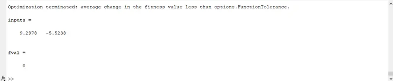
[inputs, fval] = ga(@stalagmite,2)

%End of program

(3) The ga_statistics code:

%GA Statistics

clear all                    %clear the workspace
close all                    %close all the open window
clc                          %clear the command window

%Defining our search space
x = linspace (0,0.6,150);
y = linspace (0,0.6,150);
num_cases = 100;
f = get_stalagmite(x,y);

%Study 1 - Statistical behaviour
tic
for i=1:num_cases
    [inputs, fopt(i)] = ga(@stalagmite,2);
    xopt(i) = inputs(1);
    yopt(i) = inputs(2);
end
study1_time = toc

%Plotting the graph for study 1 
figure(1)
subplot(2,1,1)
hold on
surfc (x,y,-f)        %'-f' to find maximam of the function
shading interp
plot3(xopt, yopt, -fopt,'marker','o','markersize',5,'markerfacecolor','r')
title('Unbounded inputs')
subplot(2,1,2)
plot(-fopt)            %'-fopt' to find maximam of the function
xlabel ('Iterations')
ylabel ('Funtion Minimum')


%Study 2 - Statistical behaviour - with upper and lower bound
tic
for i=1:num_cases
    [inputs, fopt(i)] = ga(@stalagmite,2,[],[],[],[],[0;0],[1;1]);
    xopt(i) = inputs(1);
    yopt(i) = inputs(2);
end
study2_time = toc

%Plotting the graph for study 2 
figure(2)
subplot(2,1,1)
hold on
surfc (x,y,-f)           %'-f' to find maximam of the function
shading interp
plot3(xopt, yopt, -fopt,'marker','o','markersize',5,'markerfacecolor','r')
title('Bounded inputs')
subplot(2,1,2)
plot(-fopt)              %'-fopt' to find maximam of the function
xlabel ('Iterations')
ylabel ('Funtion Minimum')


%Study 3 - Statistical behaviour - with icreasing GA iteration
options = optimoptions('ga');
options = optimoptions(options,'PopulationSize', 250);

tic
for i=1:num_cases
    [inputs, fopt(i)] = ga(@stalagmite,2,[],[],[],[],[0;0],[1;1],[],[],options);
    xopt(i) = inputs(1);
    yopt(i) = inputs(2);
end
study3_time= toc

%Plotting the graph for study 3
figure(3)
subplot(2,1,1)
hold on
surfc (x,y,-f)               %'-f' to find maximam of the function
shading interp
plot3(xopt, yopt, -fopt,'marker','o','markersize',5,'markerfacecolor','r')
title('Bounded inputs with modified Population size')
subplot(2,1,2)
plot(-fopt)                  %'-f' to find maximam of the function
xlabel ('Iterations')
ylabel ('Funtion Minimum')

%End of program

ERRORS:

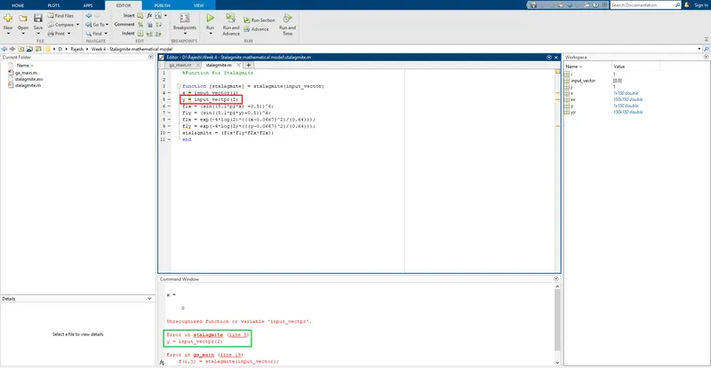
(1) Typo are the most common mistakes while writing a code.

RESULTS:

Using the GA, we created 3 case studies to find the global maxima of the function.

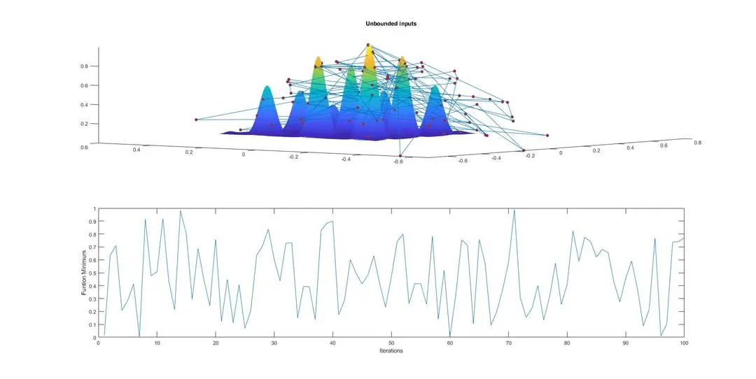
Case 1: Unbounded inputs

GA will take the population size as 50 by default and try to find the minima of the function on the surface. As we can observe the values going out of the domain and there are multiple points where it can find maxima of the function.

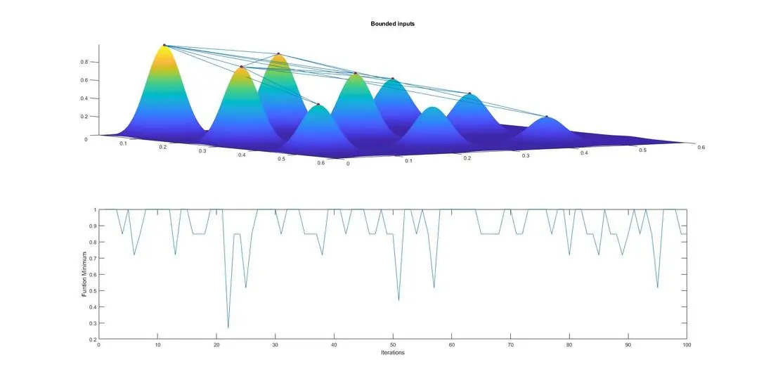
Case 2: Bounded inputs

As we can observe from the above case there are multiple points where GA finds the maxima of the function. In this case, we can constraint the boundary and set the limit for GA to find the maxima of the function under the range of `x` & `y` as defined. Still, there are multiple values from GA as maxima of the function.

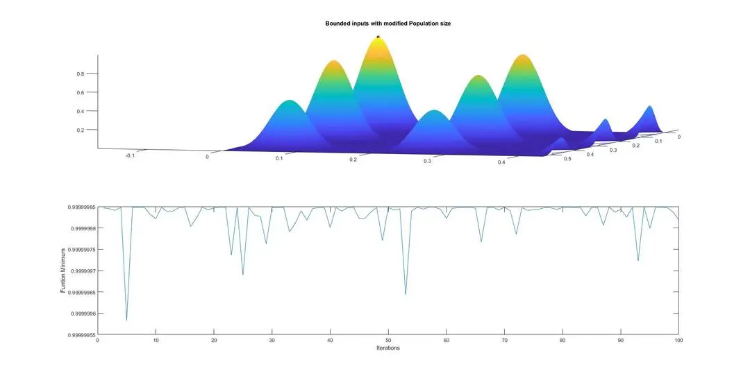
Case 3: Bounded inputs with increased population size

As in the above case, we get 4 points as the maxima of the function under the range of `x` and `y` input. In this case, we can increase the population size so that the GA get more number of samples data points to define the maxima of the function on the surface. There are three steps to optimize the increased population size.

• Selection: In this step, the parents are selected from the sample data points, the main objective of the selection process is to select the highly fit individuals.
• Cross over: It is a process of making two parents' solutions and producing the child from them.
• Mutation: It is carried out to maintain the genetic diversity from one generation of the population of the chromosomes to the next.

Workspace Output:

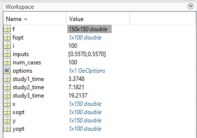
The input values of `x` & `y`:

CONCLUSION: Successfully executed the code using the Genetic Algorithm and found the global maxima of the function. Also. perform different case studies to plot the graph between F maximum vs no. of iterations.