Week 4 - CHT Analysis on Exhaust port

CHT Analysis on Exhaust port

Aim: To simulate Exhaust port by Conjugate Heat Transfer Analysis.

Introduction:

The exhaust port is passage which transport the burned mixture during produced during power stroke. These burnt gases are at high temperature and therefore be sent into the atmosphere without any issue. To facilitate this exhaust port is used.

CHT stands for conjugate heat transfer, which means heat transfer process involving an interaction of conduction within a solid body and the convection from the solid surface to fluid moving over the solid surface. Therefore, a realistic analysis of conjugate heat transfer problems necessitates the coupling of the conduction in the solid and the convection in the fluid. This is generally accomplished by satisfying the conditions of continuity in temperature and heat flux at the fluid–solid interface.

Steps followed:

These are the steps followed in setting up the simulation.

a) Geometry

b) Mesh

c) Setup

d) Results

These steps will be explained one by one in detail.

a) Geometry:

Firstly, import Ansys fluent analysis system and open geometry in it. In spaceclaim import the model file of exhaust port.

File > spaceclaim options > units > meters.

After importing the model, it looks like:

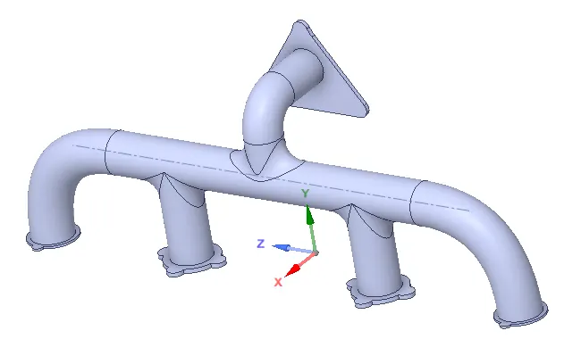
Repair > extra edges. (This removes any unwanted or extra edges in the model). In our case, the geometry was perfectly fine.

Prepare > volume extract > edge selection tool.

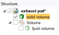
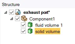
Work bench > share

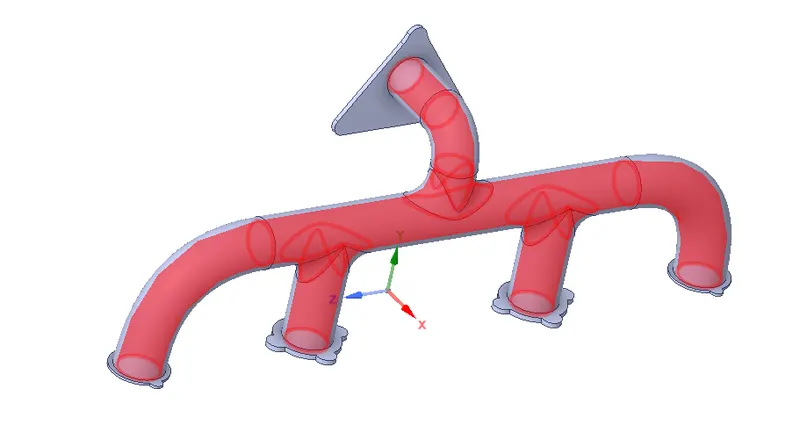
Share topology - select share option.

b) Mesh:

Open Meshing,

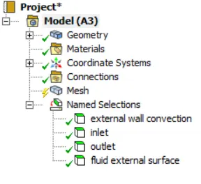
Create Named selection.

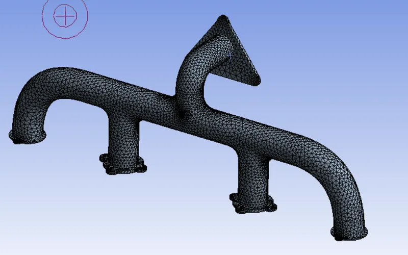
Basic Mesh:

The mesh at the interface is perfectly alligned in solid and fuid volume with out any overlapping or gaps.

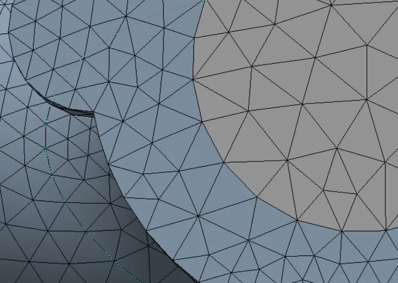
We will refine the mesh.

Inflation layers added to the outer surface of the fluid volume.

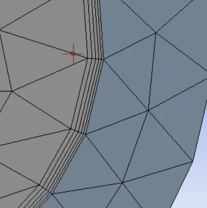
Final Refined Mesh:

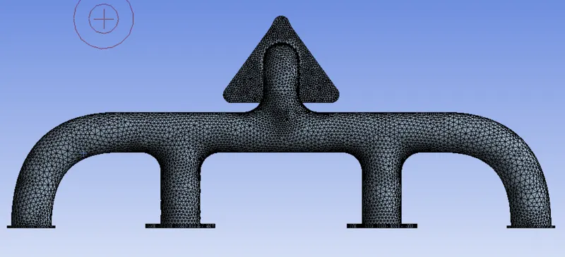
c) Setup:

In setting up the physics, we select

pressure based solver

steady state analysis

Enable energy equation

K-epsilon standard viscous model

Materials

1) for solid volume select Aluminium

2) for fluid volume select air

Input boundary conditions

velocity at inlet is 5m/s and 700K

Wall heat transfer co-efficient on the wall outer surface is 20W/m2K.

In solving,

initialize the hybrid solution.

In post-processing,

create tempertaure contour.

In solving,

Create animation of temperature contour.

Run simulation.

d) Results:

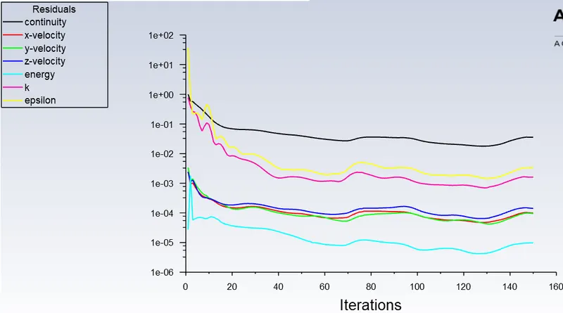
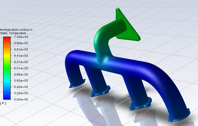
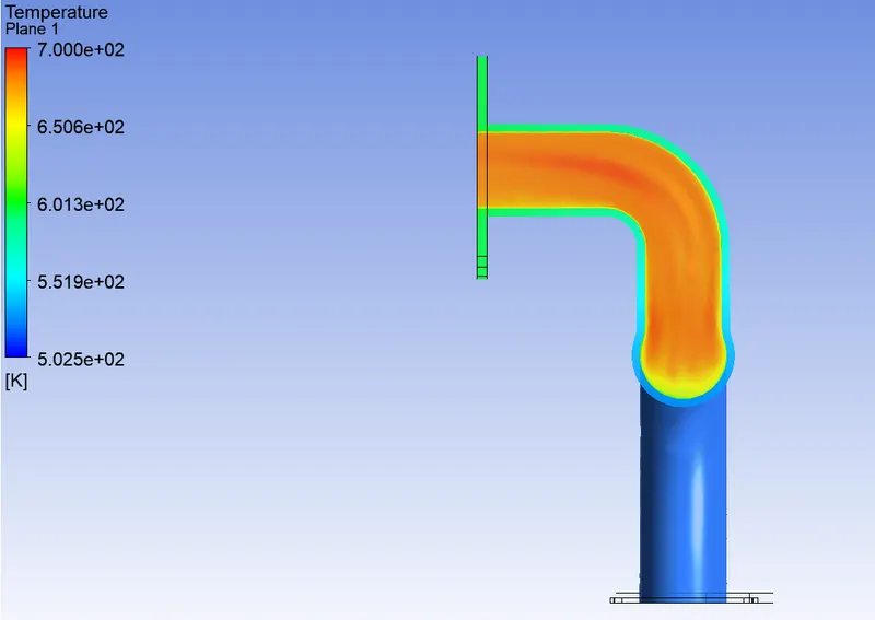
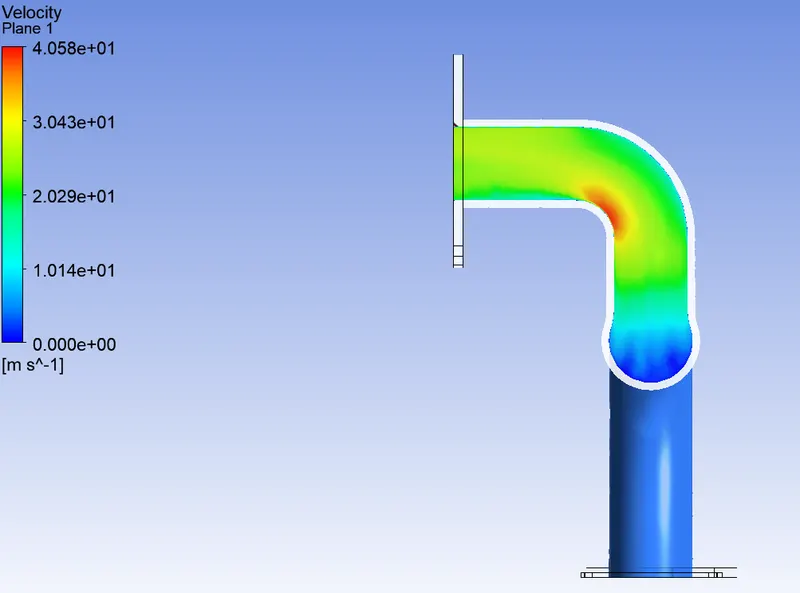
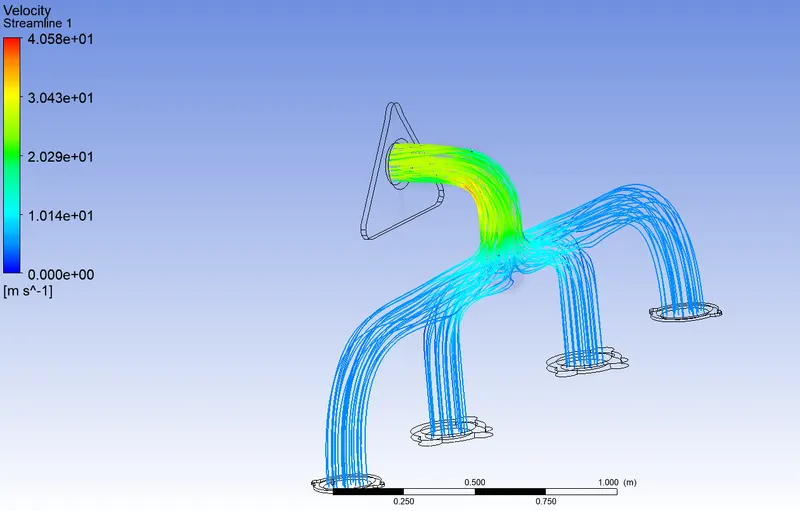
Conclusion:

y+ is a non-dimensional distance. It is often used to describe how coarse or fine a mesh is for a particular flow pattern. It is important in turbulence modeling to determine the proper size of the cells near domain walls. The turbulence model wall laws have restrictions on the y+ value at the wall. For instance, the standard K-epsilon model requires a wall y+ value between approximatly 300 and 100. A faster flow near the wall will produce higher values of y+, so the grid size near the wall must be reduced.

HTC predictions from the simulations can validated using by setting up experiment. The other way to validate is to refer to a research paper which was written based on the same experimental results. The accuracy of the predictons depend on many factors. Some of them are:

1) How well we define the boundary conditions. They should be consistent with the actual process.

2) The type of viscous model we use.

3) How well the described heat transfer co-efficient is consistent with actual heat transfer co-efficient.

In this simulation,we set up the conjugate heat transfer problem of exhaust port.