CHT Analysis on Exhaust port

Aim – To simulate Conjugate Heat Transfer Analysis on exhaust port using Ansys Fluent.

Objective –

1. Brief description on where and why CHT analysis is used?
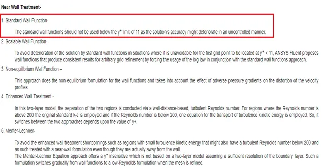
2. Justify results by maintaining appropriate y+ value for turbulence model.
3. Calculate Wall HTC and Surface HTC on inner and on surface of solid part exhaust ports?
4. Show Velocity and temperature contours in appropriate areas respectively.
5. Justify, how do verify if HTC predicted from simulations are right?
6. On what factors does the accuracy of the prediction depends?

Theory -

Conjugate heat transfer (CHT)

Conjugate heat transfer corresponds with the combination of heat transfer in solids fluids.

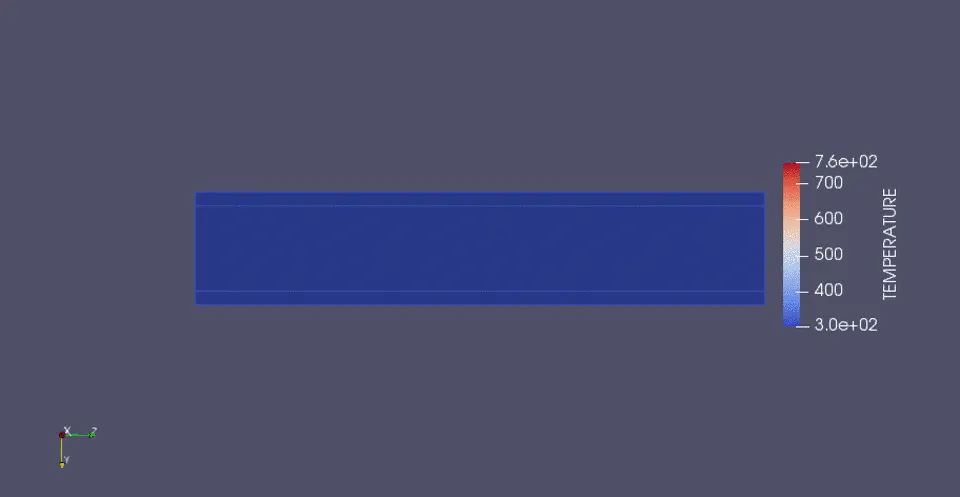
Heat Transfer in a Solid

In most cases, heat transfer in solids, if only due to conduction, is described by Fourier’s law defining the conductive heat flux, q, proportional to the temperature gradient: .

For a time-dependent problem, the temperature field in an immobile solid verifies the following form of the heat equation:

Heat Transfer in a Fluid

Due to the fluid motion, three contributions to the heat equation are included:

1. The transport of fluid implies energy transport too, which appears in the heat equation as the convective contribution. Depending on the thermal properties on the fluid and on the flow regime, either the convective or the conductive heat transfer can dominate.
2. The viscous effects of the fluid flow produce fluid heating. This term is often neglected, nevertheless, its contribution is noticeable for fast flow in viscous fluids.
3. As soon as a fluid density is temperature-dependent, a pressure work term contributes to the heat equation. This accounts for the well-known effect that, for example, compressing air produces heat.

Accounting for these contributions, in addition to conduction, results in the following transient heat equation for the temperature field in a fluid:

Conjugate Heat Transfer Applications

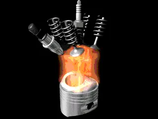
• Internal combustion engine

• Cross Flow heat temperature,
• Integrated Circuit Chips,

• HVAC
• turbocharger,
• Cooling of Electronic Devices, Burners and Combuster
• Heat transfer in fin arrays, micro-channels and ribbed passages.
• Drying of porous flat plate.

Why CHT analysis?

• Conjugate heat transfer (CHT) analysis can accurately predict heat transfer by simultaneous solving all the relevant solid and fluid flow field heat transfer processes, for example: conduction through solids, free and forced convection in the gases/fluids and thermal radiation.
• The CHT approach has an advantage over FEA thermal analysis.
• In that wall heat transfer coefficients and their local variations on surfaces are directly calculated within the model rather than based on simplified empirical calculations.
• The CHT approach therefore has benefits for those applications where heat transfer is either non-uniform or difficult to calculate empirically.

Wall Heat Transfer Coefficient and Y+ value –

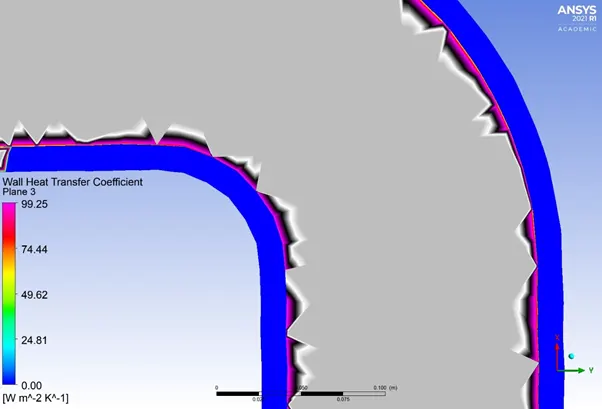
1. Wall HTC is quantity that can calculated at the first cell layer of wall adjacent to that of fluid.
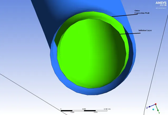
2. With inflation layer, user can notice accurate capturing of Wall HTC along the surface separating solid and fluid volumes.
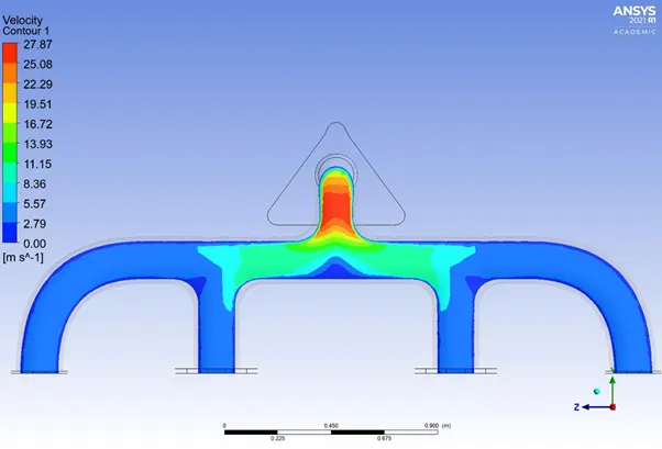
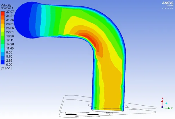
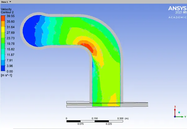
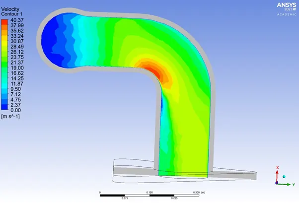
3. Maximum HTC is predicted/captured at the same location of maximum velocity.

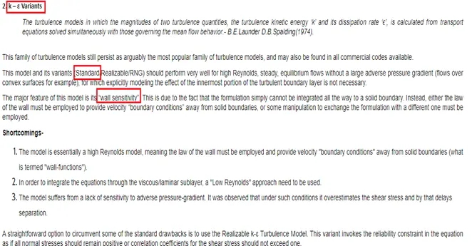
Brief about Turbulence Model used for Analysis –

Procedure-

Problem Setup –

(1) Geometry

Files → Space Claim Options → Units

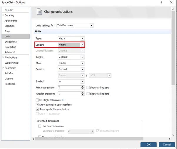
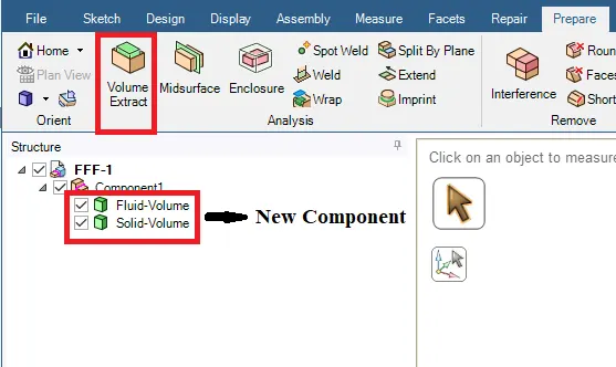
Extract the geometry in Space Claim with following procedure,

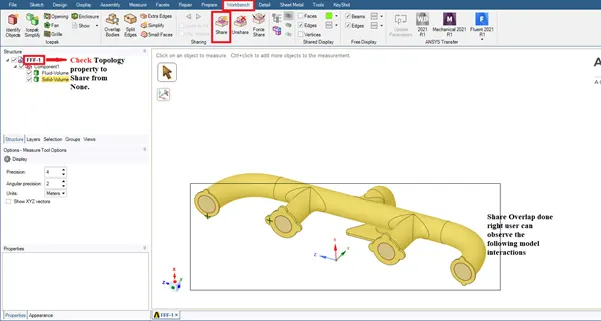
(2) Mesh Generation –

N key → Insert → Named Selection, As follows

---------------------------------------------------------------------------------------------------------------------------------------------------

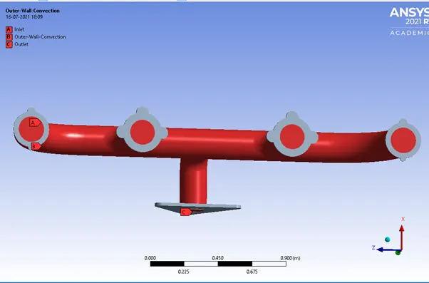
Baseline Mesh –

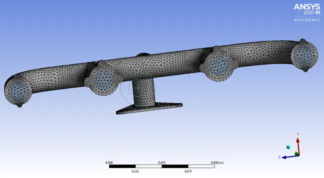
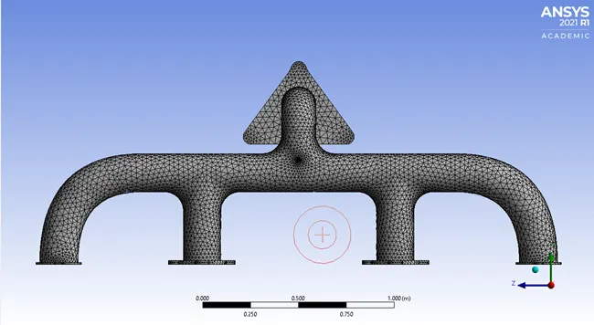
Mesh Details -

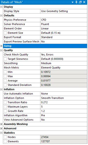
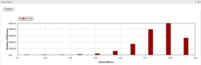
Mesh Quality Metrics -

Refinement 1 & 2 –

N key → Insert → Named Selection, As follows

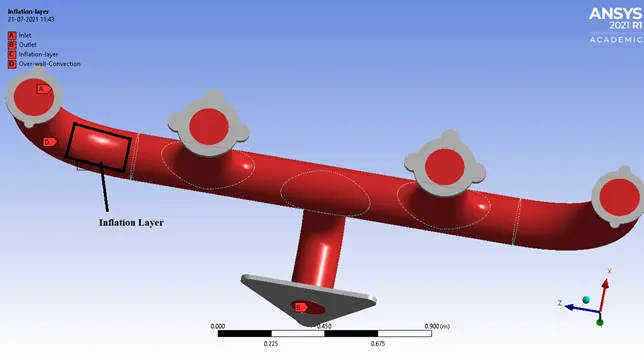
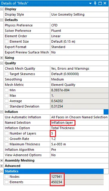
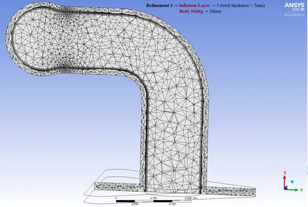
Inflation Layer –

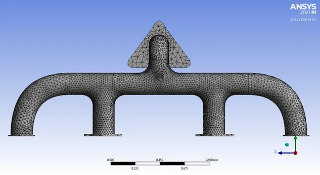
Mesh Refinement 1 –

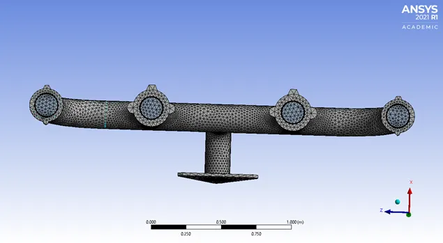
Mesh Detail –

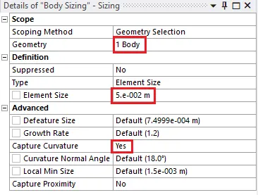
Body Sizing Details –

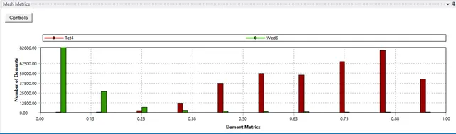
Mesh Quality Metrics –

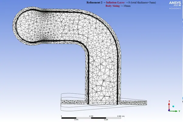
Mesh Refinement 2 –

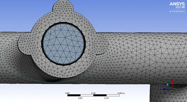
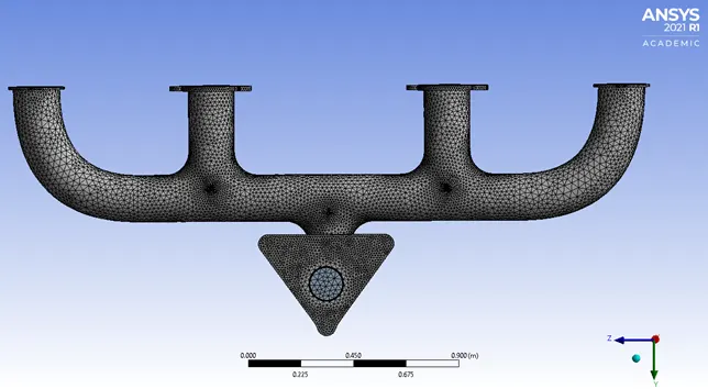
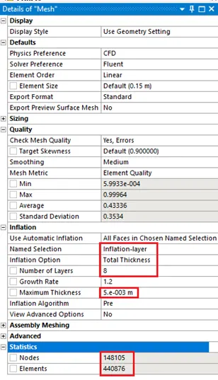
Mesh Detail –

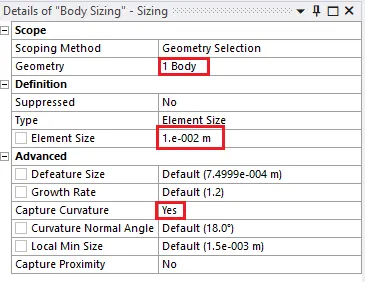
Body Sizing Details –

Mesh Quality Metrics –

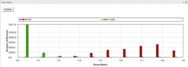
Inference from both Refinements

---------------------------------------------------------------------------------------------------------------------------------------------------

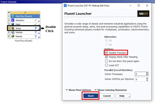
(3) Fluent Setup –

(4) Solution Setup -

1. General → Solver → Pressure-based → Time→ Steady State
2. Models → Viscous → K-epsilon → Standard Model → Standard Wall Function
3. Material → Fluid → Air → Solid → Aluminum
4. Cell Zone Conditions → fff-component_Fluid-volume → Fluid → Air

fff-component_Solid-volume → Solid → Aluminum

5. Boundary Conditions →
6. Intel (Velocity= User-defined)
7. Outlet (Gauss Pressure=1 atm)
8. Outer-wall-Convection →

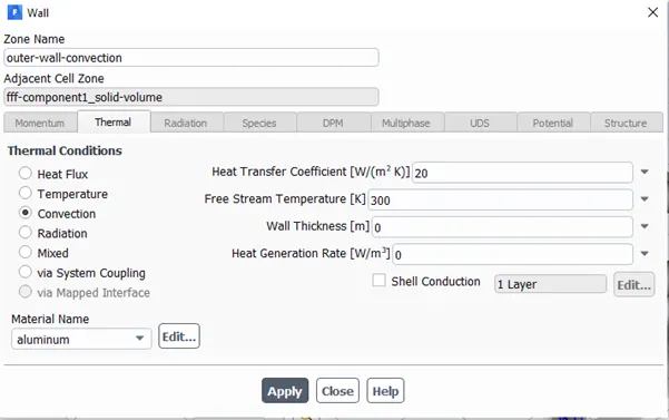
9. Wall Component → Wall Motion → Stationary → Shear Condition → No Slip

10.Inflation Layers → Coupled

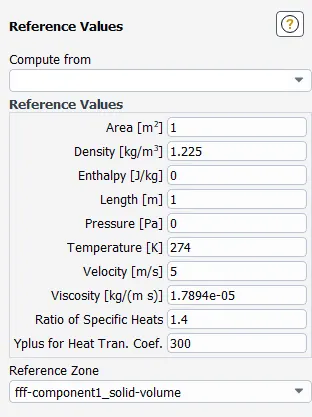
(5) Reference Values →

• Method → Scheme → Simple
• Initialize Solution → Hybrid
• Results →
• Create Contour → Velocity → Field Variable = All Named Selections
• Create Contour → Pressure → Field Variable = All Named Selections
• Create Contour → Temperature → Field Variable = All Named Selections
• Activities → Create Animation → Solution Animation → Temperature Contour
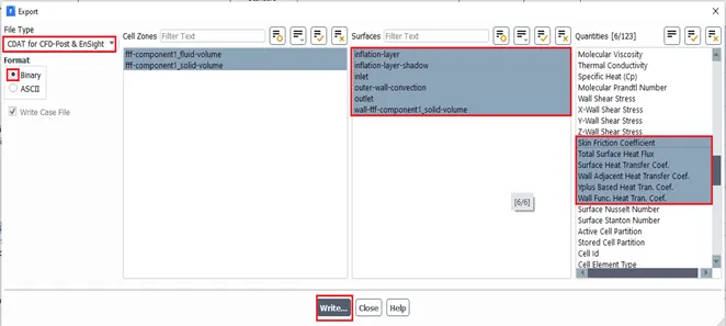
• HTC extraction Activities → Export → Solution Data →

---------------------------------------------------------------------------------------------------------------------------------------------------

Results –

Exhaust Port Baseline Results –

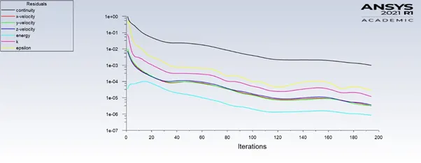
Residual Plot –

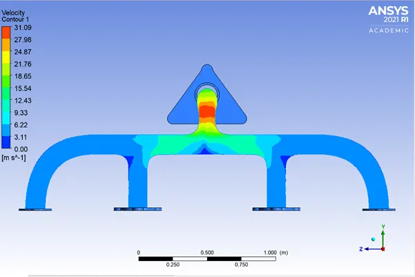
Velocity Contour –

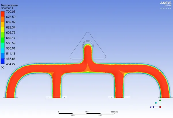
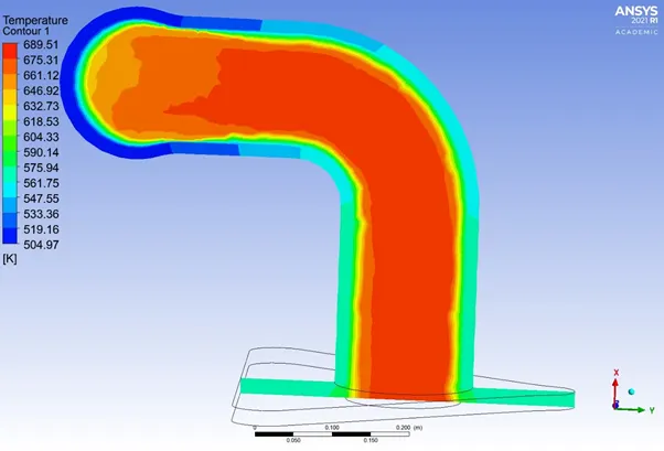
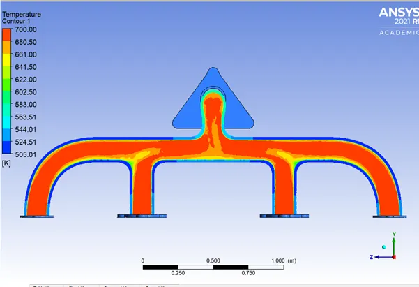
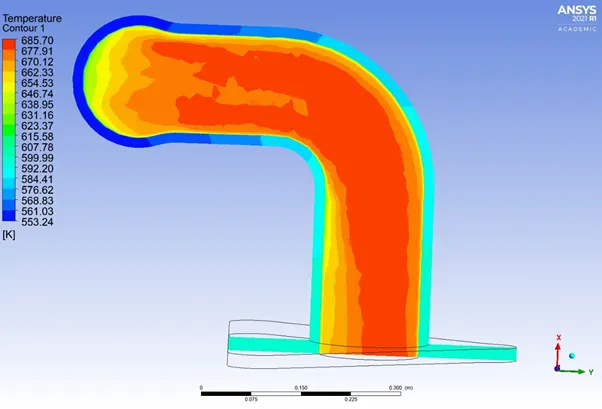
Temperature Contour –

Streamline Movement –

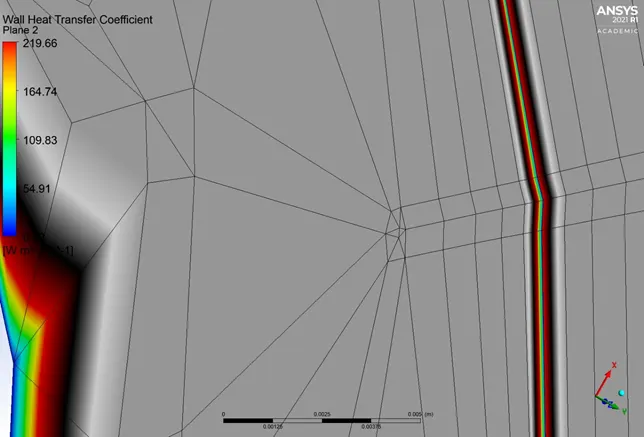
Wall Heat Transfer Coefficient –

---------------------------------------------------------------------------------------------------------------------------------------------------

Exhaust Port Refinement 1 Results –

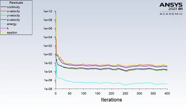
Residual Plot –

Velocity Contour –

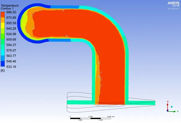
Temperature Contour –

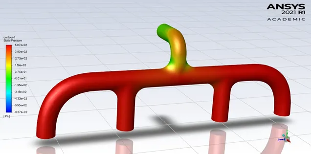
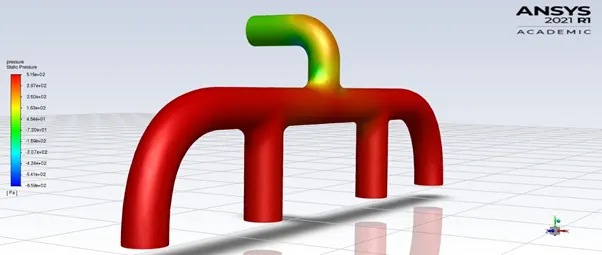
Pressure Contour –

Streamline Movement –

Wall Heat Transfer Coefficient –

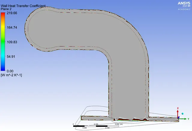
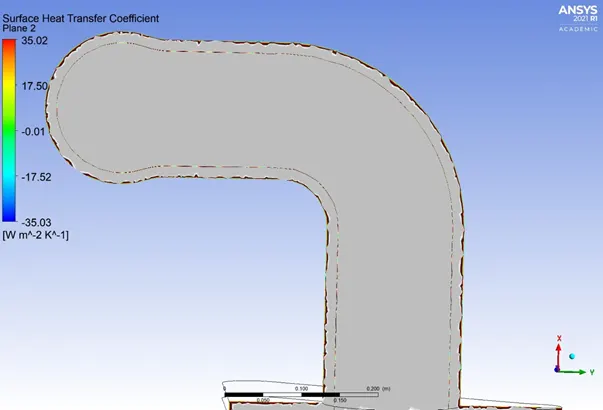
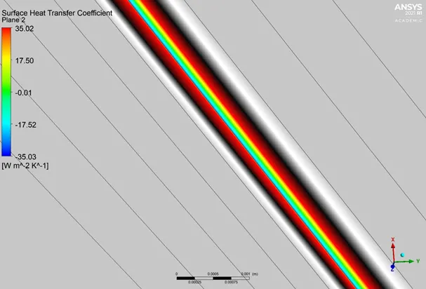
Surface Heat Transfer Coefficient –

---------------------------------------------------------------------------------------------------------------------------------------------------

Exhaust Port Refinement 2 Results –

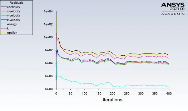
Residual Plot –

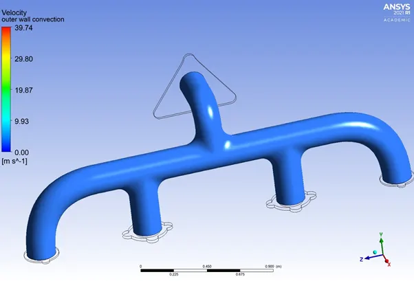
Velocity Contour –

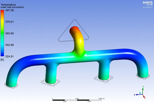
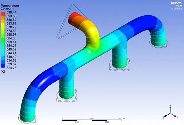
Temperature Contour –

Pressure Contour –

Streamline Movement –

Wall Heat Transfer Coefficient –

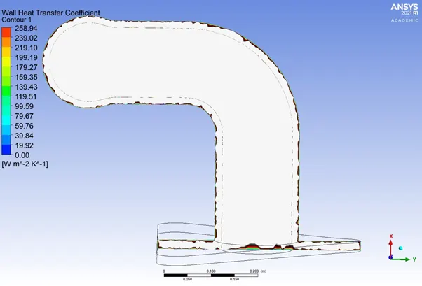
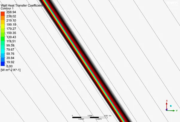
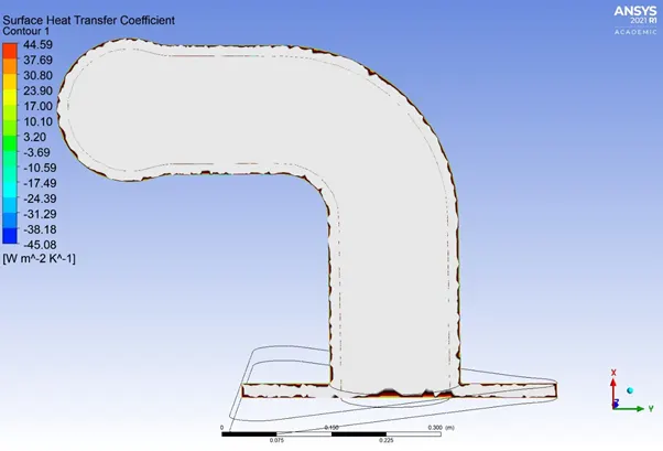
Surface Heat Transfer Coefficient –

---------------------------------------------------------------------------------------------------------------------------------------------------

Result Table –

SL. No	Analysis on Exhaust Port	Elements	Nodes	Inflation Layer	Surface HTC (W/m^2 K^-1)	Wall HTC (W/m^2 K^-1)
1	Baseline	137707	27454	Nil	21.75	99.25
2	Refinement 1	450234	127941	5	35.02	219.66
3	Refinement 2	440876	148105	8	44.59	256.94

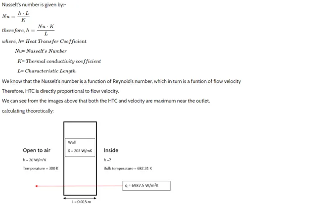
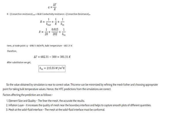
How do verify if HTC predicted from simulations are right? On what factors does the accuracy of the prediction depends?

Conclusion –

1. In case 1, mesh generated has default setting and the results captured are less accurate due to the same.
2. In case 2 ‘a’ & ‘b’, inflation created results in finer mesh around solid wall. Leading to a capturing temperature contour and HTC more accurately than case 1.
3. From above cases we notice the following results –

• Velocity tends to increase from inlet to outlet due to mass conservation and mixing of air.
• Transfer of heat from fluid to solid is high and leads to formation high velocity at the junction resulting in HTC capturing.
• The internal flow velocity and its characteristics are affected by initial velocity, pressure and physical features of geometry. Thus, CHT analysis is essential prior experimental process for better prediction product life of design component.
• As shown in the plots, the exhaust gases passing through the manifold transfers some of the heat via convection. The amount of heat transfer can be related directly with the velocity of exhaust.
• The temperature is lower where flow stagnates or is moving at the velocity. As the velocity increases, so does the Reynold’s number and the amount of heat transferred.

4. Most accurate methods to predict results is to do a comparative study of experimental and analytical results on Nusselt’s Number.
5. Otherwise, another method to verify is to validate simulation data with published experimental data.