Mid term project - Solving the steady and unsteady 2D heat conduction problem
Objective -
1. Steady state analysis & Transient State Analysis
Solve the 2D heat conduction equation by using the point iterative techniques that were taught in the class. The Boundary conditions for the problem are as follows;
Top Boundary = 600 K
Bottom Boundary = 900 K
Left Boundary = 400 K
Right Boundary = 800 K
You will implement the following methods for solving implicit equations.
1. Jacobi
2. Gauss-seidel
3. Successive over-relaxation
2. You will write code for both implicit and explicit schemes (This is for the Transient Analysis only)
3. Write a detailed explanation for your results, plots or codes without explanation will awarded zero marks.
Procedure -
We know that the steady state 2D heat equation is-
`(d^2t)/(dx^2) + (d^2t)/(dy^2) = 0`
- The above equation is a 2nd order PDE with space variable x and y
- Its elipitical in nature and requires data from all neigbhouring points to calculate the value of function at that point.
On discretization of the above euation we get -
`(T_L -2T_P +T_R)/(trianglex^2) + (T_T -2T_P +T_B)/(triangley^2) =0`
Then find `T_P``
`T_P = 1/k *((T_L-2T_P+T_R)/(trianglex^2) + (T_T-2T_P+T_B)/(triangley^2))`
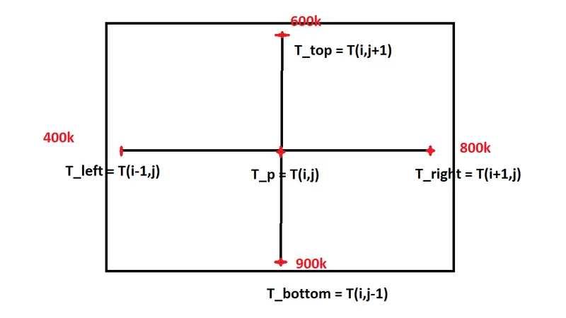
From the above representation we can compute the equation for iterative solvers like Jacobi. GS, SOR.
Jacobi iterative formulae -
`T_(i,j) ^(n+1) = 1/k*((T_(i-1,j)^n+T_(i+1,j)^n)/(trianglex^2) + (T_(i,j-1)^n+T_(i,j+1)^n)/(triangley^2))`
Gauss Siedal iterative formulae -
`T_(i,j) ^(n+1) = 1/k*((T_(i-1,j) ^(n+1)+T_(i+1,j)^n )/(trianglex^2) + (T_(i,j-1) ^(n+1)+T_(i,j+1)^n)/(triangley^2))`
SOR iterative formulae -
`T_(i,j) ^(n+1) = T_(i,j) ^n(1 - omega) + omegaT_(gs)(i,j)`
where T_gs = Gauss Seidal iterative solver
Transient State Analysis
We know that 2D heat equa. in transient state is -
`(dT)/(dt) = ((d^2T)/(dx^2) + (d^2T)/(dy^2))`
- This equation has a elpitical and hyperbolic part
- For further discretization we need to follow Forward Time and Central Space scheme.
`(T^(n+1)-T^n)/(trianglet) = alpha((T_(i+1,j) -2T_(i,j)+T_(i-1,j))^n/(trianglex^2)+(T_(i,j+1) -2T_(i,j)+T_(i,j-1))^n/(triangley^2))`
Explicit Scheme -
`T_(i,j)^(n+1) = (1-2k1-2k2)T_(i,j)^n + k1*(T_(i+1,j)^n + T_(i-1,j)^n) + k2*(T_(i,j+1)^n)+T_(i,j-1)^n)`
Where,
`k1=alpha(dt/(dx^2))`
`k2=alpha(dt/(dy^2))`
Implicit Scheme -
`T_(i,j)^(n+1) =(T_(i,j)^n + k1*(T_(i+1,j)^(n+1) + T_(i-1,j)^(n+1)) + k2*(T_(i,j+1)^(n+1)+T_(i,j-1)^(n+1)))/ (1-2k1-2k2)`
Code -
- Steady State Scheme Function Creation -
Jacobi Function
function jacobi_iter_steady(L,ny,tol)
%const
L=1;
ny=20;%Grid point size
nx=ny;
x=linspace(0,L,nx);
y=linspace(L,0,ny);
dx=L/(nx-1);
dy=L/(ny-1);

%Assigning BC
T_R=800;
T_L=400;
T_T=600;
T_B=900;

%Temperature Matrix
T=298*ones(nx,ny);
T(1,:)=T_B;
T(nx,:)=T_T;
T(:,1)=T_L;
T(:,ny)=T_R;

Told=T;
error= 9e9;
k=2*(dx^2+dy^2)/(dx^2*dy^2);

 %Convergence Loop
 jacobi_iter=1;
 while(error>tol)
     %Space Loop
      for i=2:(nx-1)
          for j=2:(ny-1)
              term1=((Told(i-1,j)+Told(i+1,j))/(dx^2));
              term2=((Told(i,j-1)+Told(i,j+1))/(dy^2));
              T(i,j)= 1/k*(term1 + term2);
          end
      end
    error=max(max(abs(Told-T)));
    Told=T;  % Updating ild values
    jacobi_iter=jacobi_iter+1;

    %Create a Contour Plot
    figure(1)
    [C,h]=contourf(x,y,T);
    set(gca,'YDIR','reverse');
    colorbar
    colormap(jet);
    clabel(C,h);
    xlabel('X axis');
    ylabel('Y axis');
    title_text=sprintf(['Solving 2D steady state heat equ. using'....
        ' Jacobi iterative solvern No. of grid point =%d;'....
        'total iteration = %d'],nx,jacobi_iter);
    title(title_text);
    pause(0.00003);
 end
end
Gauss Seidal Function
function gs_iter_steady(L,ny,tol)

%const
L=1;
ny=20;%Grid point size
nx=ny;
x=linspace(0,L,nx);
y=linspace(L,0,ny);
dx=L/(nx-1);
dy=L/(ny-1);

%Assigning BC
T_R=800;
T_L=400;
T_T=600;
T_B=900;

%Temperature Matrix
T=298*ones(nx,ny);
T(1,:)=T_B;
T(nx,:)=T_T;
T(:,1)=T_L;
T(:,ny)=T_R;

Told=T;
k=2*(dx^2+dy^2)/(dx^2*dy^2);

error= 9e9;


 %Convergence Loop
 gs_iter=1;
 while(error>tol)
     %Space Loop
      for i=2:(nx-1)
          for j=2:(ny-1)
              term1=((T(i-1,j)+Told(i+1,j))/(dx^2));
              term2=((T(i,j-1)+Told(i,j+1))/(dy^2));
              T(i,j)= 1/k*(term1 + term2);
          end
      end
    error=max(max(abs(Told-T)));
    Told=T;  % Updating ild values
    gs_iter=gs_iter+1;

    %Create a Contour Plot
    figure(1)
    [C,h]=contourf(x,y,T);
    set(gca,'YDIR','reverse');
    colorbar
    colormap(jet);
    clabel(C,h);
    xlabel('X axis');
    ylabel('Y axis');
    title_text=sprintf(['Solving 2D steady state heat equ. using'....
        ' GS iterative solvern No. of grid point =%d;'....
        'total iteration = %d'],nx,gs_iter);
    title(title_text);
    pause(0.00003);
 end
end
SOR Function
function SOR_iter_steady(L,ny,tol)

%const
L=1;
ny=20;%Grid point size
nx=ny;
x=linspace(0,L,nx);
y=linspace(L,0,ny);
dx=L/(nx-1);
dy=L/(ny-1);

%Assigning BC
T_R=800;
T_L=400;
T_T=600;
T_B=900;

%Temperature Matrix
T=298*ones(nx,nx);
T(1,:)=T_B;
T(nx,:)=T_T;
T(:,1)=T_L;
T(:,ny)=T_R;

Told=T; %Copying the value of T
k=2*(dx^2+dy^2)/(dx^2*dy^2);

error= 9e9;
Omega=1.7;  %Relaxation Factor

 %Convergence Loop
 sor_iter=1;
 while(error>tol)
     %Space Loop
      for i=2:(nx-1)
          for j=2:(ny-1)
              term1=((T(i-1,j)+Told(i+1,j))/(dx^2));
              term2=((T(i,j-1)+Told(i,j+1))/(dy^2));
              T(i,j)=(1-Omega)*Told(i,j)+ Omega*(1/k*(term1 + term2));
          end
      end
    error=max(max(abs(Told-T)));
    Told=T;  % Updating ild values
    sor_iter=sor_iter+1;

    %Create a Contour Plot
    [C,h]=contourf(x,y,T);
    set(gca,'YDIR','reverse');
    colorbar
    colormap(jet);
    clabel(C,h);
    xlabel('X axis');
    ylabel('Y axis');
    title_text=sprintf(['Solving 2D steady state heat equ. using'...
        ' SOR iterative solver n No. of grid point =%d;'...
        'total iteration = %d'],nx,sor_iter);
    title(title_text);
    pause(0.00003);
 end
end
Main Program -
close all
clc

%Initial conditions
L=1;%Length of the domain
ny=20;%Grid point size
nx=ny;
tol= 1e-4; % Tolerance

iterative_solver=input('1)Jacobi 2)Gauss Seidal 3)SOR nEnter an option for the type of solver you would like to use: n');

if iterative_solver==1
    jacobi_iter_steady(L,ny,tol);
elseif iterative_solver==2
    gs_iter_steady(L,ny,tol);
elseif iterative_solver==3
    SOR_iter_steady(L,ny,tol);
end
Transient State Explicit Scheme -
close all
clc

%const
L=1;
ny=10;%Grid point size
nx=ny;
dt=0.001;
x=linspace(0,L,nx);
y=linspace(L,0,ny);
dx=L/(nx-1);
dy=L/(ny-1);


%Assigning BC
T_R=800;
T_L=400;
T_T=600;
T_B=900;

%Temperature Matrix
T=298*ones(nx,ny);
T(1,:)=T_B;
T(nx,:)=T_T;
T(:,1)=T_L;
T(:,ny)=T_R;

T(1,1)=650;
T(1,end)=850;
T(end,1)=500;
T(end,end)=700;


tol=1e-4;
error= 9e9;
alpha=1.5;
k1=alpha*(dt/dx^2);
k2=alpha*(dt/dy^2);

[X,Y]=meshgrid(x,y);
Told=T;

CFL=k1+k2
unsteady_iter=1;

tic
for nt=1:1400
 %Convergence Loop
 while(error>tol)
     %Space Loop
      for i=2:(nx-1)
          for j=2:(ny-1)
              term1=Told(i-1,j)-2*Told(i,j)+Told(i+1,j);
              term2=Told(i,j-1)-2*Told(i,j)+Told(i,j+1);
              T(i,j)=Told(i,j)+(k1*term1)+(k2*term2);
          end
      end
    error=max(max(abs(Told-T)));
    Told=T;  % Updating ild values
    unsteady_iter=unsteady_iter+1;
    %Create a Contour Plot
    figure(1)
    [C,h]=contourf(X,Y,T);
    set(gca,'YDIR','reverse');
    colorbar
    colormap(jet);
    clabel(C,h);
    xlabel('X axis');
    ylabel('Y axis');
    title_text=sprintf(['Unsteady Explicit Iteration= %d'...
        'nNo of grid points= %d; dt=%g'],unsteady_iter,nx,dt);
    title(title_text);
    pause(0.03);
 end
end

time_taken= toc
Transient State Implicit Scheme -
Jacobi Function
function transient_implicit_jacobi(L,n,tol,t,dt)
%Initial conditions
nx=n;
ny=nx;
x=linspace(0,L,nx);
y=linspace(L,0,ny);
dx=L/(nx-1);
dy=L/(ny-1);
n_t=t/dt;
alpha=1;

%Assigning BC
T_R=800;
T_L=400;
T_T=600;
T_B=900;

%Temperature Matrix
T=ones(nx,ny);
T(1,:)=T_B;
T(nx,:)=T_T;
T(:,1)=T_L;
T(:,ny)=T_R;
T_old=T;
T_prev=T;
n_iter=1;

k1=alpha*dt/dx^2;
k2=alpha*dt/dy^2;

%Time Loop
for k=1:n_t
    error =1;
    %Convergence Loop
    while(error>tol)
        %Space Loop
        for i=2:(nx-1)
          for j=2:(ny-1)
              %Implicit Jacobi scheme
              T(i,j)=(T_prev(i,j)+k1*(T_old(i-1,j)+T_old(i+1,j))+k2*(T_old(i,j-1)+T_old(i,j+1)))/(1+2*k1+2*k2);
          end
        end
        %Convergence error
        error=max(max(abs(T-T_old)));
        %Updating old value
        T_old=T;
        n_iter=n_iter+1;
    end
    %Updating previous value
    T_prev=T;

end

%Plotting a contour Plot
 figure(1)
    [C,h]=contourf(x,y,T);
    set(gca,'YDIR','reverse');
    colorbar
    colormap(jet);
    clabel(C,h);
    xlabel('X axis');
    ylabel('Y axis');
    title_text=sprintf(['Solving 2D steady state heat equ. implicitly'....
        ' using Jacobi iterative solvern No. of grid point =%d;'....
        'total iteration = %d'],n,n_iter);
    title(title_text);
    pause(0.0001);
end
Gauss Seidal Function -
function transient_implicit_GS(L,n,tol,t,dt)
%Initial conditions
nx=n;
ny=nx;
x=linspace(0,L,nx);
y=linspace(L,0,ny);
dx=L/(nx-1);
dy=L/(ny-1);
n_t=t/dt;
alpha=1;

%Assigning BC
T_R=800;
T_L=400;
T_T=600;
T_B=900;

%Temperature Matrix
T=ones(nx,ny);
T(1,:)=T_B;
T(nx,:)=T_T;
T(:,1)=T_L;
T(:,ny)=T_R;
T_old=T;
T_prev=T;
gs_iter=1;

k1=alpha*dt/dx^2;
k2=alpha*dt/dy^2;

%Time Loop
for k=1:n_t
    error =1;
    %Convergence Loop
    while(error>tol)
        %Space Loop
        for i=2:(nx-1)
          for j=2:(ny-1)
              %Implicit GS scheme
              T(i,j)=(T_prev(i,j)+k1*(T(i-1,j)+T_old(i+1,j))+k2*(T(i,j-1)+T_old(i,j+1)))/(1+2*k1+2*k2);
          end
        end
        %Convergence error
        error=max(max(abs(T-T_old)));
        %Updating old value
        T_old=T;
        gs_iter=gs_iter+1;
    end
    %Updating previous value
    T_prev=T;

end

%Plotting a contour Plot
  figure(1)
    [C,h]=contourf(x,y,T);
    set(gca,'YDIR','reverse');
    colorbar
    colormap(jet);
    clabel(C,h);
    xlabel('X axis');
    ylabel('Y axis');
    title_text=sprintf(['Solving 2D steady state heat equ. implicitly'....
        ' using GS iterative solvern No. of grid point =%d;'....
        'total iteration = %d'],n,gs_iter);
    title(title_text);
    pause(0.0001);
end
SOR Function -
function transient_implicit_SOR(L,n,tol,t,dt)
%Initial conditions
nx=n;
ny=nx;
x=linspace(0,L,nx);
y=linspace(L,0,ny);
dx=L/(nx-1);
dy=L/(ny-1);
n_t=t/dt;
alpha=1;

%Assigning BC
T_R=800;
T_L=400;
T_T=600;
T_B=900;

%Temperature Matrix
T=ones(nx,ny);
T(1,:)=T_B;
T(nx,:)=T_T;
T(:,1)=T_L;
T(:,ny)=T_R;
T_old=T;
T_prev=T;
sor_iter=1;
T_gs=zeros(nx,ny);
omega=1.5;

k1=alpha*dt/dx^2;
k2=alpha*dt/dy^2;

%Time Loop
for k=1:n_t
    error =1;
    %Convergence Loop
    while(error>tol)
        %Space Loop
        for i=2:(nx-1)
          for j=2:(ny-1)
              %Implicit SOR scheme
              T_gs(i,j)=(T_prev(i,j)+k1*(T(i-1,j)+T_old(i+1,j))+k2*(T(i,j-1)+T_old(i,j+1)))/(1+2*k1+2*k2);
              T(i,j)=T_prev(i,j)*(1-omega)+omega*T_gs(i,j);
          end
        end
        %Convergence Error
        error=max(max(abs(T-T_old)));
        %Updating old value
        T_old=T;
        sor_iter=sor_iter+1;
    end
    %Updating previous value
    T_prev=T;
end

%Plotting a contour Plot
    figure(1)
    [C,h]=contourf(x,y,T);
    set(gca,'YDIR','reverse');
    colorbar
    colormap(jet);
    clabel(C,h);
    xlabel('X axis');
    ylabel('Y axis');
    title_text=sprintf(['Solving 2D steady state heat equ. implicitly'....
        ' using SOR iterative solvern No. of grid point =%d;'....
        'total iteration = %d'],n,sor_iter);
    title(title_text);
    pause(0.0001);
end
Main Program -
close all
clc

L=1;   %Domain length of x & y
n=20;  %Grid point along x & y
nx=n;
ny=nx;
tol=1e-4; %Convergence critrion
t=0.2;    %desireed time of temperature distribution
dt=1e-4;  %Time step size

iterative_solver=input('1)Jacobi 2)Gauss Seidal 3)SOR nEnter an option for the type of solver you would like to use: n');

if iterative_solver==1
    transient_implicit_jacobi(L,nx,tol,t,dt);
elseif iterative_solver==2
   transient_implicit_GS(L,n,tol,t,dt);
elseif iterative_solver==3
  transient_implicit_SOR(L,n,tol,t,dt);
end
Output -
Steady state 2D heat equation -
1)Jacobi 2)Gauss Seidal 3)SOR
Enter an option for the type of solver you would like to use:
1
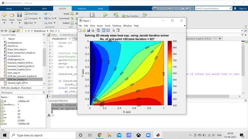
1)Jacobi 2)Gauss Seidal 3)SOR
Enter an option for the type of solver you would like to use:
2
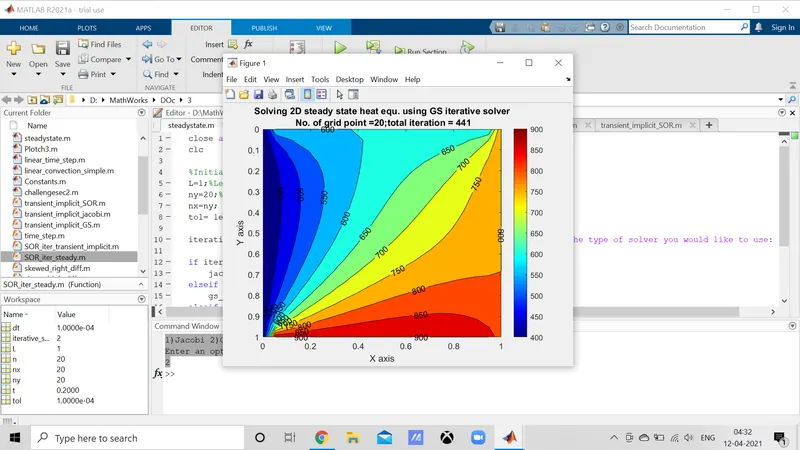
1)Jacobi 2)Gauss Seidal 3)SOR
Enter an option for the type of solver you would like to use:
3
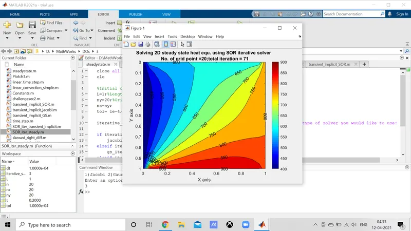
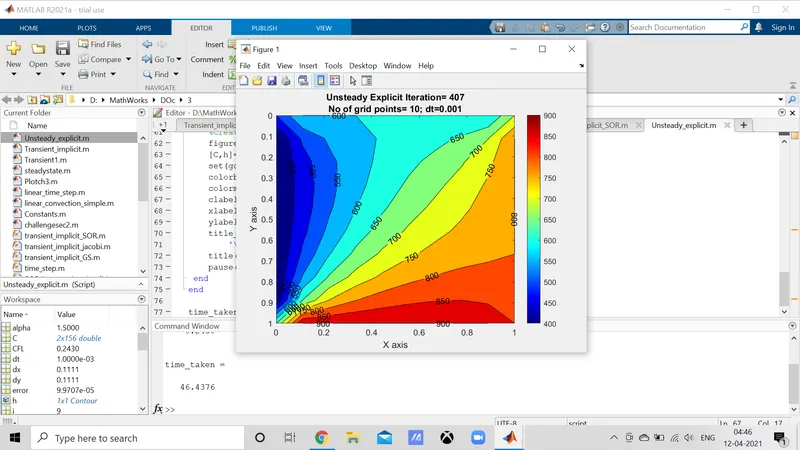
Transient state 2D heat equation (Explicit Scheme) -
CFL =
0.2430
time_taken =
46.4376
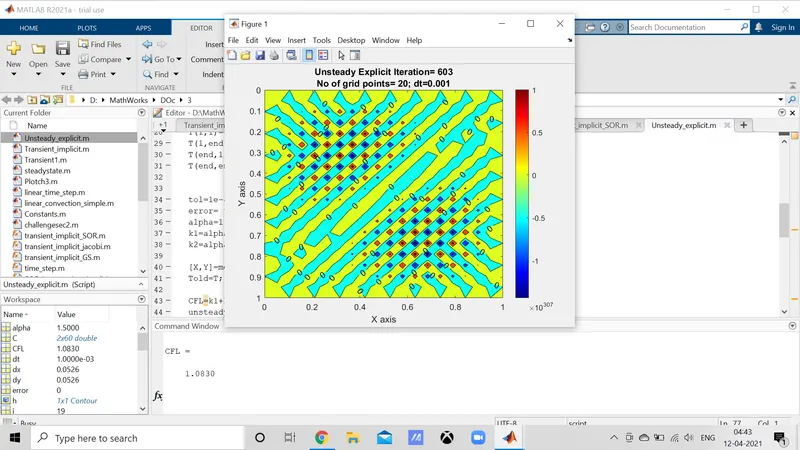
Blown Up Explicit Scheme -
CFL =
1.0830
time_taken =
137.9360
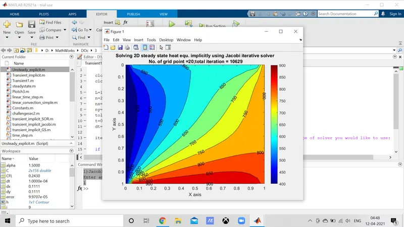
Transient 2D heat equation (Implicit Scheme)
1)Jacobi 2)Gauss Seidal 3)SOR
Enter an option for the type of solver you would like to use:
1
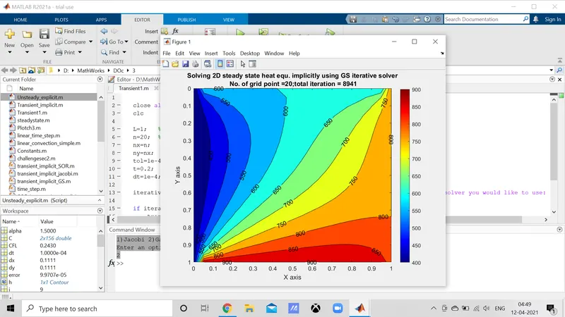
1)Jacobi 2)Gauss Seidal 3)SOR
Enter an option for the type of solver you would like to use:
2
1)Jacobi 2)Gauss Seidal 3)SOR
Enter an option for the type of solver you would like to use:
3
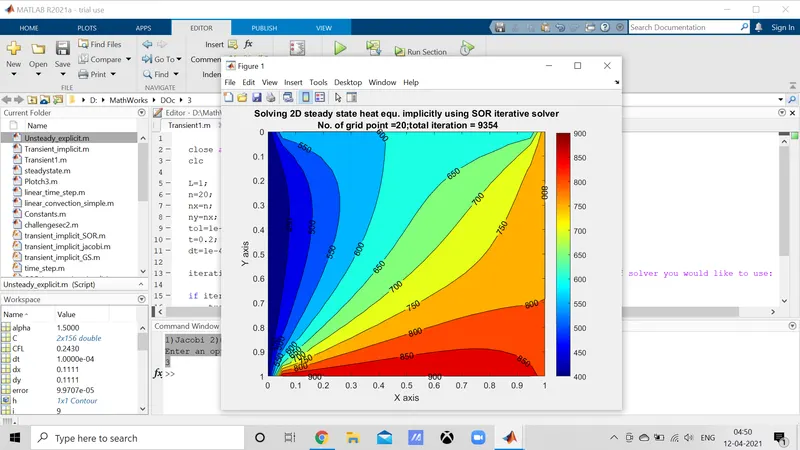
Inference -
- From the above plots ,it can be found that explicit scheme is the fastest to solve the transient 2D heat equation as we are not bothered about iteration and convergence.
- Advantage of Explicit scheme is that it doesn't need guess value and convergence criteria.
- But explicit scheme has to be stricitly governed by CFL stability condition
- i.e `CFL <= 0.5`to offer better stability .
- If we see the Implicit Scheme are slower and more complicated than explicit scheme , since we are using guess value and iteration for convergence at each time step
- However, they are unconditionally stable for any choice of dtwith respect to dx.
- In implicit plot we notice that Jacobi method took the most number of iteration to converge followed by SOR(omega =1.5) and then Gauss Seidal.
- In steady state metrhod, there is no time loop and the results converge within we iterations.
- Whereas in the implicit method, intoducing of time loop results converge to run with a large number of iterations.
- Computation time is more for transient solver as it is a function of both time and position.
- Whereas, in case of steady state solver its a function of only position.
- Successive Over Relaxation method converges with less number of iteration and computational time.