Deriving 4th order approximation of a 2nd order derivative using Taylor Table method

Objective -

Derive the following 4th order approximations of the second-order derivative.

1. Central difference

2. Skewed right-sided difference

3. Skewed left-sided difference

Once you have done this, write a program in Matlab to evaluate the second-order derivative of the analytical function exp(x)*cos(x) and compare it with the 3 numerical approximations that you have derived.

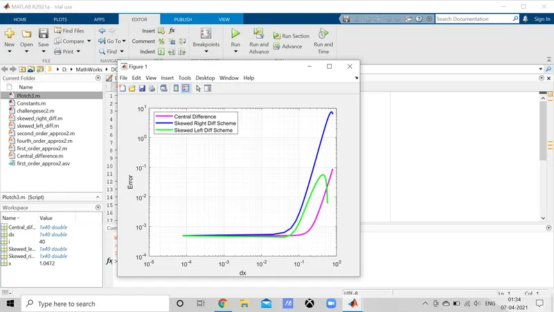
Provide a plot that compares the absolute error between the above-mentioned schemes

In your own words, describe why a skewed scheme is useful? What can a skewed scheme do that a CD scheme cannot?

Procedure -

1. Central Difference Scheme -

We know that : No of nodes = order of approximation + order of derivative -1 = 2+4-1=5

Central difference = `(a(f(i-2))+b(f(i-1))+c(f(i))+d(f(i+1))+e(f(i+2)))/(dx^2)`

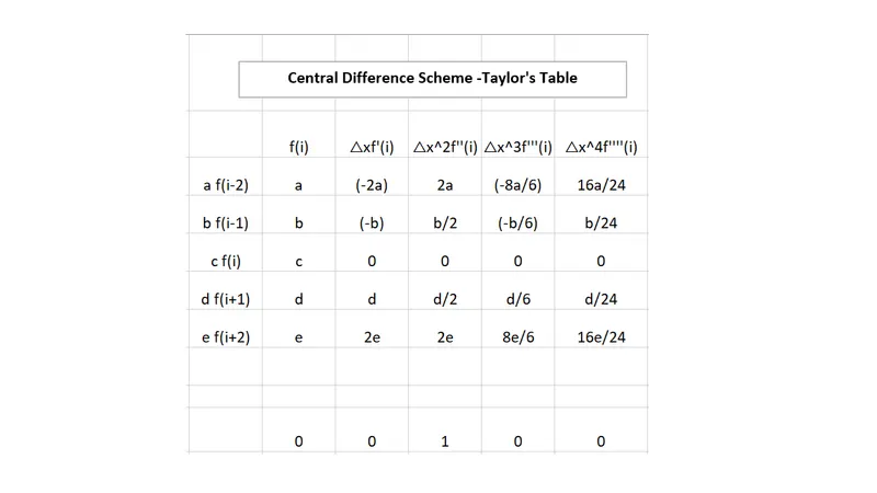
Central_diff= `((-0.0833*exp(x-2*dx)*cos(x-2*dx))+(1.3333*exp(x-dx)*cos(x-dx))+(-2.5000*exp(x)*cos(x))+(1.3333*exp(x+dx)*cos(x+dx))+(-0.0833*exp(x+2*dx)*cos(x+2*dx)))/dx^2;`

2. Skewed Right Sided Difference Scheme -

We know that : No of nodes = order of approximation + order of derivative = 2+4 = 6

SRDS= (a(f(i))+b(f(i+1))+c(f(i-2))+d(f(i-3))+e(f(i-4))+g(f(i-5)))/(dx^2)

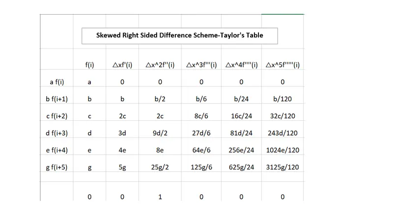
skewed_rightside_diff=`((3.7500*exp(x)*cos(x))+(-12.8333*exp(x+dx)*cos(x+dx))+(17.8333*exp(x+2*dx)*cos(x+2*dx))+(-13.0000*exp(x+3*dx)*cos(x+3*dx))+(5.0833*exp(x+4*dx)*cos(x+4*dx))+(-0.8333*exp(x+5*dx)*cos(x+5*dx)))/dx^2;`

3. Skewed Left Sided Difference Scheme -

We know that : No of nodes = order of approximation + order of derivative = 2+4 = 6

SLDS= (g(f(i-5))+e(f(i-4))+d(f(i-3))+c(f(i-2))+b(f(i-1))+a(f(i)))/(dx^2)

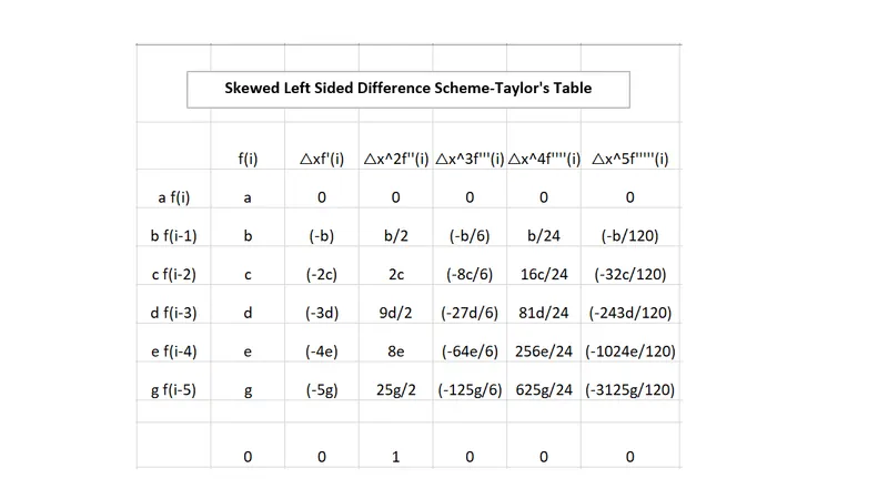
skewed_leftside_diff= `((-0.8333*exp(x-5*dx)*cos(x-5*dx))+(5.0833*exp(x-4*dx)*cos(x-4*dx))+(-13.0000*exp(x-3*dx)*cos(x-3*dx))+(17.8333*exp(x-2*dx)*cos(x-2*dx))+(-12.8333*exp(x-dx)*cos(x-dx))+(3.7500*exp(x)*cos(x)))/dx^2;`

We also know that `f(x) = exp(x)*cos(x)`

that implies `f'(x)= e^x*cos(x) - e^x*sin(x) = -2*exp(x)*sin(x)`

Thus Analytical Function = `-2*exp(x)*sin(x)`

Code -

function out_1 = skewed_right_diff(x,dx)

%Function = exp(x)*cos(x)
%Skewed right sided function = f'(x) = e^x*cos(x) - e^x*sin(x)= -2*exp(x)*sin(x)
analytical_diff= -2*exp(x)*+sin(x);

%SRDS= (a(f(i))+b(f(i+1))+c(f(i-2))+d(f(i-3))+e(f(i-4))+g(f(i-5)))/(dx^2)
skewed_rightside_diff= ((3.7500*exp(x)*cos(x))+(-12.8333*exp(x+dx)*cos(x+dx))+(17.8333*exp(x+2*dx)*cos(x+2*dx))+(-13.0000*exp(x+3*dx)*cos(x+3*dx))+(5.0833*exp(x+4*dx)*cos(x+4*dx))+(-0.8333*exp(x+5*dx)*cos(x+5*dx)))/dx^2;

out_1=(analytical_diff - skewed_rightside_diff );

end

function out_2 = skewed_left_diff(x,dx)

%Function = exp(x)*cos(x)
%Skewed left sided function = f'(x) = e^x*cos(x) - e^x*sin(x)= -2*exp(x)*sin(x)
analytical_diff= -2*exp(x)*sin(x);

%SLDS= (g(f(i-5))+e(f(i-4))+d(f(i-3))+c(f(i-2))+b(f(i-1))+a(f(i)))/(dx^2)
skewed_leftside_diff= ((-0.8333*exp(x-5*dx)*cos(x-5*dx))+(5.0833*exp(x-4*dx)*cos(x-4*dx))+(-13.0000*exp(x-3*dx)*cos(x-3*dx))+(17.8333*exp(x-2*dx)*cos(x-2*dx))+(-12.8333*exp(x-dx)*cos(x-dx))+(3.7500*exp(x)*cos(x)))/dx^2;

out_2=( analytical_diff - skewed_leftside_diff );

end

function out_3 = Central_difference(x,dx)

%Function = exp(x)*cos(x)
%central function = f'(x) = e^x*cos(x) - e^x*sin(x)> f''(x)=-2*exp(x)*sin(x)
analytical_diff= -2*exp(x)*sin(x);

%Cental Diference = (a(f(i-2))+b(f(i-1))+c(f(i))+d(f(i+1))+e(f(i+2)))/(dx^2)
central_diff= ((-0.0833*exp(x-2*dx)*cos(x-2*dx))+(1.3333*exp(x-dx)*cos(x-dx))+(-2.5000*exp(x)*cos(x))+(1.3333*exp(x+dx)*cos(x+dx))+(-0.0833*exp(x+2*dx)*cos(x+2*dx)))/dx^2;

out_3= (analytical_diff - central_diff );

end

clear all
close all
clc

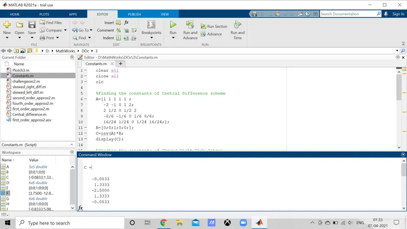
%Finding the constants of Central Difference scheme
A=[1 1 1 1 1 ;
   -2 -1 0 1 2;
   2 1/2 0 1/2 2
   -8/6 -1/6 0 1/6 8/6;
   16/24 1/24 0 1/24 16/24;];
B=[0;0;1;0;0;];
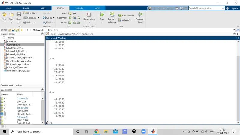
C=inv(A)*B;
display(C);

%Finding the constants of Skewed Right Side Scheme
D=[1 1 1 1 1 1;
   0 1 2 3 4 5;
   0 1/2 2 9/2 8 25/2;
   0 1/6 8/6 9/2 64/6 125/6;
   0 1/24 16/24 81/24 256/24 625/24;
   0 1/120 32/120 243/120 1024/120 3125/120;];
E=[0;0;1;0;0;0;];
F=inv(D)*E;
display(F);

%Finding the constants of Skewed Left Side Scheme
G=[1 1 1 1 1 1;
  -5 -4 -3 -2 -1 0;
   25/2 8 9/2 2 1/2 0;
   125/6 64/6 9/2 8/6 1/6 0;
   625/24 256/24 81/24 16/24 1/24 0;
   3125/120 1024/120 243/120 32/120 1/120 0;];
H=[0;0;1;0;0;0;];
J=inv(G)*H;
display(J);

clear all
close all
clc



%Assigning values foe x and dx to plot the solution of error
x = pi/3;
dx = linspace(pi/4,pi/40000,40); 

%Loop to call the functions
for i =1:length(dx)
    Central_diff_error(i)= Central_difference(x,dx(i));
    Skewed_rightsided_error(i) = skewed_right_diff(x,dx(i));
    Skewed_leftsided_error(i)= skewed_left_diff(x,dx(i));
    
end

%ploting graph of error vs dx for SLDS,SRDS,CD of 4th order approximation
%of 2nd order derivative

figure(1)
loglog(dx,Central_diff_error,'m','linewidth',2);
hold on
grid on
loglog(dx,Skewed_rightsided_error,'b','linewidth',2);
hold on
loglog(dx,Skewed_leftsided_error,'g','linewidth',2);
xlabel('dx');
ylabel('Error');
legend('Central Difference','Skewed Right Diff Scheme','Skewed Left Diff Scheme','location','best');

Observation -

In your own words, describe why a skewed scheme is useful? What can a skewed scheme do that a CD scheme cannot?

• If we result wise then central difference scheme gives us more accurate solution than skewed difference scheme.
• But Central difference scheme has its own limitation i.e it requires both sides data of node or boundary (like mid point thereom for a side of triangle).
• Whereas this drawback is overcome by skewed difference scheme as the approxmiation solution can be found from either sides of nodes or boundary
• Example of such skewed difference scheme approach is followed in this question.