FVM Literature Review

Questions -

1. What is Finite Volume Method(FVM)?
2. Write down the major differences between FDM & FVM?
3. Need for interpolation schemes and flux limiters in FVM?

Finite Volume Method-

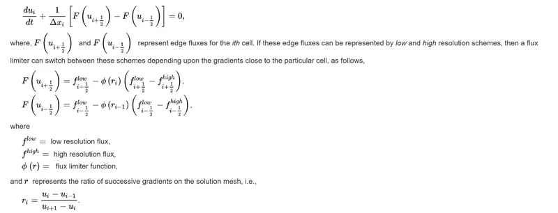
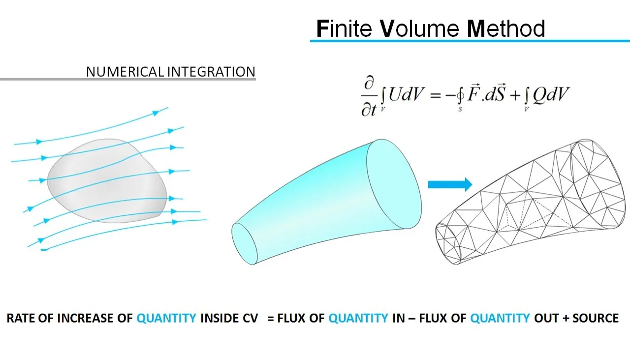
It is method for representing & evaluating PDE's in the form of algebraic equations.In FVM, the volume integral in PDE that contains divergernce term are converted into surface integral using divergernce theorem. These terms are then evaluated as flux terms for each finite volume. The flux entering a given volume is almost identical to that of adjacent volume, these methods are conservative.

Advantage of FVM is that it is easily formulated to allow for unstructured meshes. Commerical software is based on the FVM method because of unstructured mesh. Easy for solving complex problems over the other methods.

In FVM instead of writing equations for single volume, we write the equation for entire volume.Also for considered volume no assumption are made for the shape of the volume.Inside a single entity volume the fow, flow quantity, energy,mass,momentum is conserved.This is called Finite Volume Representation.

Consider 1-D steady state heat conduction equation, The governing equation is given by

`d/dx(kdt/dx)+S=0`_________(1)

Where , S is source term.

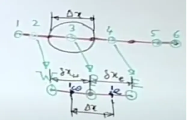
From the above above figure we divide the domain into sub-domain i.e nothing but Control Volume.

Where in 2,3,4,5 are the centriod of the control volume and 1,6 are BC.

Here we take in consideration a single control volume whose centre is 3-

• Centriod of grid point is P
• E & W are denoted by East and West. They are the immediate negihbour of P for 1-D
• `trianglex`is the lenght of the control volume.
• Lowe case alphabets denote Faces and Upper case denote Grid Point.

Now use integrate (1) for further discretization

`int_w^e d/dx(kdt/dx)dx+int_w^e Sdx=0`

`(k(dT)/dx)_e-(k(dT)/dx)_w + Strianglex=0`

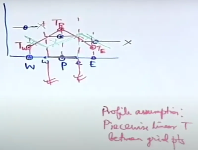
`k_e(T_e-T_p)/(deltax_e)-k_w(T_p-T_w)/(deltax_w)+Strianglex=0`

Simplifying,

`(k_e/(deltax_e)+k_w/(deltax_w))T_p=k_e/(deltax_e)*T_e+k_w/(deltax_w)*T_w+S*trianglex=0`

Symbolic writing the above equation -

`a_PT_P=a_ET_E+a_WT_W+f`

Where, `a_E=k_e/(deltax_e)`

`a_W=k_w/(deltax_w)`

`a_P=a_E+a_W`& `f=S*trianglex`

The above is FVM discretized equation from governing equation

Difference between FVM and FDM -

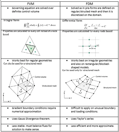
Need for interpolation schemes and flux limiters in FVM-

• The use of interpolation schemes to approximate the property values located at the boundaries of the control volumes are necessary when FVM is applied, using as interpolation nodes the correspondent properties located at the center of the adjacent control volumes.
• Low-order schemes are commonly considered, due to their numerical stability and readiness of implementation.
• However, these schemes demand the use of a high degree of refinement of the meshes due their lack of accuracy. Low order interpolation schemes can lead to inaccurate results provoked by numerical diffusion effects.
• Alternatively, high-order interpolation schemes produce more accurate solutions with low computational costs.
• When applying high-order schemes to nonuniform meshes, it is necessary to keep in mind several precautions in the development of interpolation formulas, since interpolation schemes were originally developed for uniform meshes .

Different ways of interpolation are-

1. Upwind Interpolation scheme
2. Linear Interpolation scheme
3. Hybrid Interpolation scheme
4. Quadratic Upwind Interpolation scheme

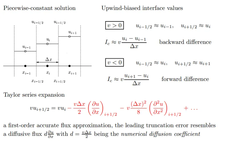
Upwind Interpolation Scheme-

This interpolation scheme is equvilanent in using forward or backward finite differencing approxination (depends on the flow direction) . Its the first order accurate scheme and is numerically diffusive with coefficient of numerical diffusion.

Linear interpolation scheme -

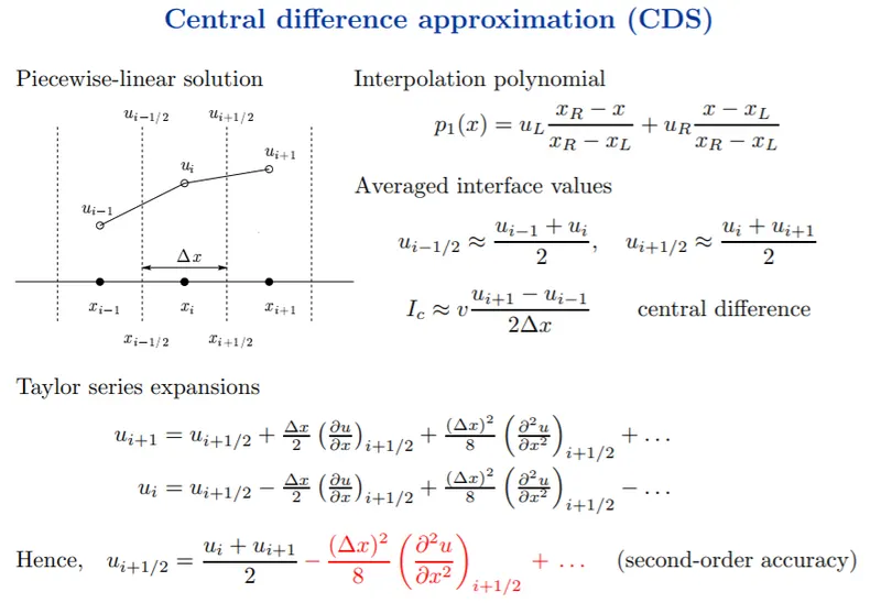
The value of the control volume of its face centre approximae to the values of near two computational nodes. This location at 'e' on cartesin grid, the value is approximed by -

`f_e=f_E(lamdae)+f_P(1-lamdae)`

`lamda_e=(x_e-x_p)/(x_E-x_P)`

The linear interpolation scheme is equivalent to the use of central difference formula of first order derivative , and this is also termed as central differencing scheme(CDS).

This scheme is second derivative and may also produce oscillatory solution.

Hybrid Interpolation Scheme-

This scheme is a combination of Upwind and Linear interpolation scheme. The cartesin grid is given by-

`phi_f=psi*phi_(ud)+(1-psi)*phi_(cd)`

Where.

`phi_f`= Value of the variable at face

`phi_(ud)`= Value of variable at face (Upwind differencing scheme)

`phi_(cd)`= Value of variable at face (Central differencing scheme)

`psi`= Function of Blend to switch between Schemes

Quadratic Interpolation Scheme-

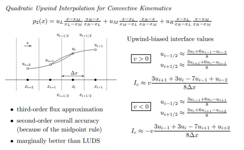
This interpolation scheme is of 3rd order scheme it is derived from Polynomial fiting.The quadratic interpolation scheme on cartesin scheme is given by

`phi_e=6/8phi_U+3/8phi_D-1/8phi_(UU)`

Where U,D,UU denote the first stream, downstream and second stream node respectively depending on the flow direction.

QUICK scheme is prone to oscillatory solution due its #rd order scheme.

Flux Limiters

In solving the convective fields, one can find discontiunity and schocks in the results. In higher order, we notice that the oscillatory motion is more and thus leads the solution to be unstable.To obtain highly accurate and oscillation free results we need to use flux limiters function .

This function provides a smooth region over the flow and maintains the first oder accuracy.

Flux limiters are usually used to obtain total variation diminishing(TVD)