Simulation of a 1D Super-sonic nozzle flow simulation using Macormack Method

QUES- In this challenge you are going to simulate the isentropic flow through a quasi 1D subsonic-supersonic nozzle. You will derive both the conservation and non-conservation forms of the governing equations and sovle them using the MacCormack's technique. You need to determine the steady-state temperature distribution for the flow-field variables and investigate the difference between the two forms of governing equations by comparing their solutions.

Objective-

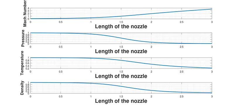
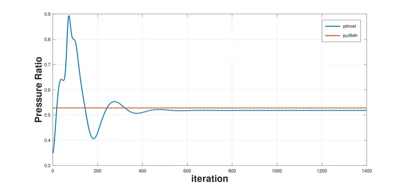
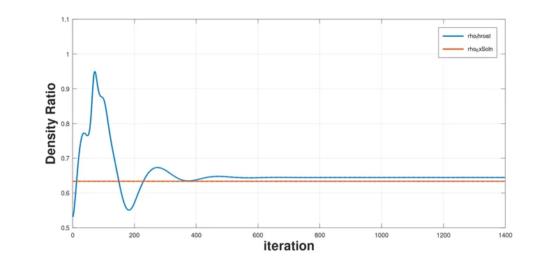
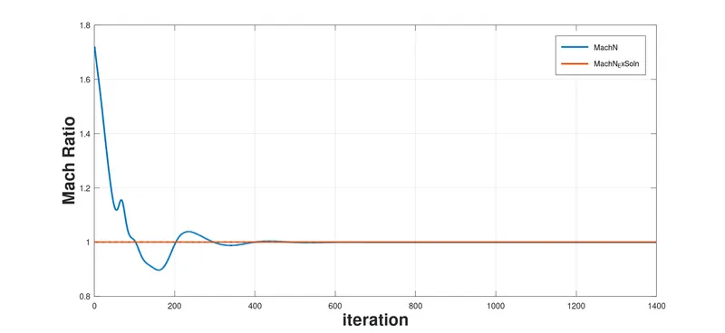
1. Steady-state distribution of primitive variables inside the nozzle
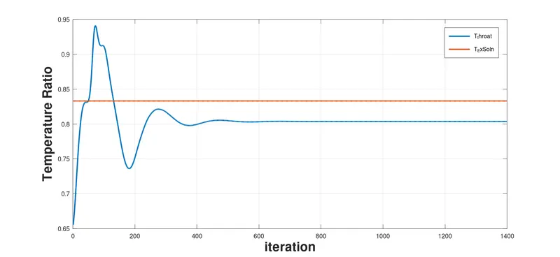
2. Time-wise variation of the primitive variables
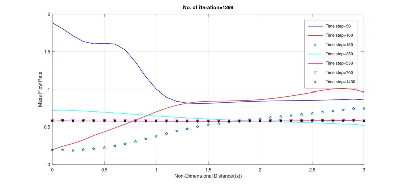
3. Variation of Mass flow rate distribution inside the nozzle at different time steps during the time-marching process
4. Comparison of Normalized mass flow rate distributions of both forms

Procedure -

Non-Dimensional Form

• Calculate initial variable density,area,velocity and temperature.
• The time loop has iteration range upto 1400.
• Further on use differentiation to solve for density,velocity and temperature. Inorder, to get the energy,momentum and continuity equations using Foward Scheme and Backward Scheme respectively.
• Update the solutions after forward scheme - `v(j)=(v(j)+((dv)/dt)_p(j))*dt`
• Similarly after correctors step, find the average of predicator and corrector step and also update the solution -
• `((drho)/dt)_(avg)(m)=0.5*(((drho)/dt)_p(m)+ ((drho)/dt)_c(m))`
• `rho(m)=(rho_(old)(m)+((drho)/dt)_(avg)(m))*dt`
• Then plot mass flow rate = `rho*area*velocity`

Equation for Non-dimensional form

Continunity Eq-

`((drho)/dt)_p(j)= -(rho(j)*(dv)/dx) - (rho(j)*v(j)*(da)/dx) - (v(j)*(drho)/dx)`

Momentum Eq-

`((dv)/dt)_p(j)= -((v(j)*(dv)/dx)- ((1/gamma)*((dt)/dx + ((T(j))/(rho(j)))*(drho)/dx)))`

Energy Eq-

`((dT)/dt)_p(j)= -(v(j)*(dt)/dx) -((gamma-1)*T(j)*((dv)/dx + (v(j)*(da)/dx)))`

Conservative Form-

• Calculate initial variable density,area,velocity and temperature.
• The time loop has iteration range upto 1400.
• Calculate the fluex F1,F2,F3 and source term J2.
• Differentiate for predicators step using forward scheme and correctors step using backward scheme.
• Similarly, update after predicators step
• `U1(j)=(U1(j)+((dU1)/dt)_p(j))*dt`
• Find the average and update after correctors step.
• `(dU1)/dt(i)=0.5*(((dU1)/dt)_p(i)+((dU1)/dt)_c(i))`
• `U1(i)=(U1_(old)(i)+((dU1)/dt)(i))*dt`
• Then plot mass flow rate = `rho*area*velocity`

Equation for Conservative Form-

`U1=rho*a`
`U2=rho*a.v`
`U3=rho*a*((T/(gamma-1))+((0.5*gamma)*(v^2)))`

`f1=U2`
`f2=((U2^2)/(U1))+(((gamma-1)/gamma)*(U3-((gamma/2)*(U2^2))/(U1)))`
`f3=((gamma*U2.*U3)/(U1)) - ((gamma*(gamma-1)*((U2^3))/(2*(U1^2))))`

`(df1)/dx=(f1(j+1)-f1(j))/dx;`
`(df2)/dx=(f2(j+1)-f2(j))/dx; (df3)/dx=(f3(j+1)-f3(j))/dx;(da)/dx=(a(j+1)-a(j))/dx;`
`J2=(1/gamma)*rho*T*(da)/dx`

Continunity Eq-

`((dU1)/dt)_p=-(df1)/dx`

Momentum Eq-

`((dU2)/dt)_p=-(((df2)/dx)+J2)`

Energy Eq-

`((dU3)/dt)_p=-(df3)/dx`

Code -

%Conservative Form of Equations

clear all
close all
clc

%cell points
n=31;
x=linspace(0,3,n);
dx=x(2)-x(1);

%initial condition
a=1+2.2*(x-1.5).^2;
n_throat=find(a-1<0.001);
iter=0;
gamma=1.5;
C=0.5;
nt=1400;

for d=1:n
    
    if (x(d)>=0 && x(d)<0.5)
        rho(d)=1;
        T(d)=1;
    elseif (x(d)>=0.5 && x(d)<1.5)
        rho(d)=1-(0.366*(x(d)-0.5));
        T(d)=1-(0.167*(x(d)-0.5));
    elseif (x(d)>=1.5 && x(d)<=3)
        rho(d)=0.634-(0.3879*(x(d)-1.5));
        T(d)=0.833-(0.3507*(x(d)-1.5));
    end
    
end
v=0.59./(rho.*a);
MFR_I=rho.*a.*v;
%rho=rho_I;
%T=T_I;
%v=v_I;
U1_I=rho.*a;
U2_I=rho.*a.*v;
U3_I=rho.*a.*((T/(gamma-1))+((0.5*gamma)*(v.^2)));

U1=U1_I;
U2=U2_I;
U3=U3_I;

% for p=1:n
%  dt_a(p)=C*dx/(T_I(p)^0.5+v_I(p));
% end
% dt=min(dt_a);

%Time Loop
for k=1:1400
    
    dt = min((C*dx)./((T.^0.5) + v));
    %   Dt=T_I.^0.5;
    %   dt=min(C*(dx./(Dt+v_I)));
    %solution vectors
    U1_old=U1;
    U2_old=U2;
    U3_old=U3;
    
    %flux vectors
    f1=U2;
    f2=((U2.^2)./U1)+(((gamma-1)/gamma)*(U3-((gamma/2)*(U2.^2))./U1));
    f3=((gamma*U2.*U3)./U1) - ((gamma*(gamma-1)*((U2.^3))./(2*(U1.^2))));
    
    %Space Loop
    %Predictors Step
    for j=2:n-1
        df1_dx(j)=(f1(j+1)-f1(j))/dx;
        df2_dx(j)=(f2(j+1)-f2(j))/dx;
        df3_dx(j)=(f3(j+1)-f3(j))/dx;
        da_dx(j)=(a(j+1)-a(j))/dx;
        J2(j)=(1/gamma)*rho(j)*T(j)*(da_dx(j));  %Source term
        
        %Continuity equation
        dU1_dt_p(j)=-df1_dx(j);
        %Momentum equation
        dU2_dt_p(j)=-(df2_dx(j))+J2(j);
        %Energy equation
        dU3_dt_p(j)=-df3_dx(j);
        
        %Updating the solution
        U1(j)=U1(j)+(dU1_dt_p(j)*dt);
        U2(j)=U2(j)+(dU2_dt_p(j)*dt);
        U3(j)=U3(j)+(dU3_dt_p(j)*dt);
    end
    
    %Variable value
    rho_p=U1./a;
    v_p=U2./U1;
    T_p=(gamma-1)*((U3./U1)-((gamma/2)*(v_p.^2)));
    
    %Correctors step
    %flux vectors
    f1=U2;
    f2=((U2.^2)./U1)+(((gamma-1)/gamma)*(U3-((gamma/2)*(U2.^2))./U1));
    f3=((gamma*U2.*U3)./U1) - ((gamma*(gamma-1)*((U2.^3))./(2*(U1.^2))));
    
    for j=2:n-1
        df1_dx(j)=(f1(j)-f1(j-1))/dx;
        df2_dx(j)=(f2(j)-f2(j-1))/dx;
        df3_dx(j)=(f3(j)-f3(j-1))/dx;
        da_dx(j)=(a(j)-a(j-1))/dx;
        J2(j)=(1/gamma)*rho(j)*T(j)*da_dx(j);    %Source term
        
        %Continuity equation
        dU1_dt_c(j)=-df1_dx(j);
        %Momentum equation
        dU2_dt_c(j)=-df2_dx(j) +J2(j);
        %Energy equation
        dU3_dt_c(j)=-df3_dx(j);
    end
    for i=2:n-1
        %compute the average time derivative
        dU1_dt(i)=0.5*(dU1_dt_p(i)+dU1_dt_c(i));
        dU2_dt(i)=0.5*(dU2_dt_p(i)+dU2_dt_c(i));
        dU3_dt(i)=0.5*(dU3_dt_p(i)+dU3_dt_c(i));
        
        %Final solution update
        
        U1(i)=U1_old(i)+dU1_dt(i)*dt;
        U2(i)=U2_old(i)+dU2_dt(i)*dt;
        U3(i)=U3_old(i)+dU3_dt(i)*dt;
    end
    %Apply the boundary condition
    %Inlet
    U1(1)=a(1);
    U2(1)=2*U2(2)-U2(3);
    U3(1)=U1(1)*((T(1)/(gamma-1)) + ((gamma/2)*(U2(1)/U1(1))^2));
    
    %Outlet
    U1(n)=(2*U1(n-1))-U1(n-2);
    U2(n)=(2*U2(n-1))-U2(n-2);
    U3(n)=(2*U3(n-1))-U3(n-2);
    
    %Analysing the properties at throat of nozzle
    rho=U1./a;
    v=U2./U1;
    T=(gamma-1)*((U3./U1)-((gamma/2)*(v.^2)));
    MachN=(v./(T.^0.5));
    p=rho.*T;
    MFR=rho.*a.*v;
    
    
    
    iter=iter+1;
end


figure(6)
subplot(4,1,1)
plot(x,MachN);
xlabel('Length if the nozzle');
ylabel('Mach Number');
grid minor;
subplot(4,1,2)
plot(x,p);
xlabel('Length if the nozzle');
ylabel('Pressure');
grid minor;
subplot(4,1,3)
plot(x,T);
xlabel('Length if the nozzle');
ylabel('Temperature');
grid minor;
subplot(4,1,4)
plot(x,rho);
xlabel('Length if the nozzle');
ylabel('Density');
grid minor;

-----------------------------------------------------------------------------------------------------------------

%Non-conservative form of Equations

clear all
close all
clc

%cell points
n=31;
x=linspace(0,3,n);
dx=x(2)-x(1);

%initial condition 
rho_I=1-0.3146*x;
T_I=1-0.2314*x;
v_I=(0.1+1.09*x).*T_I.^(0.5);
a=1+2.2*(x-1.5).^2;
n_throat=find(a-1<0.001);
iter=0;
gamma=1.5;
C=0.5;

rho=rho_I;
T=T_I;
v=v_I;

nt=1400;
for w=1:n
dt_initial(w)=(C*(dx./((T_I(w).^0.5) + v_I(w))));
end
dt=min(dt_initial);
simulation_time=(nt-1)*dt;
t=0:dt:simulation_time;

%Time Loop
for k=1:nt
      
    rho_old=rho;
    v_old=v;
    T_old=T;   
    
    %Space Loop
    %Predicator step
    for j=2:n-1
        dv_dx=(v(j+1)-v(j))/dx;
        drho_dx=(rho(j+1)-rho(j))/dx;
        dt_dx=(T(j+1)-T(j))/dx;
        da_dx=(log(a(j+1))-log(a(j)))/dx;
        
        %Continuity equation
        drhodt_p(j)= -(rho(j)*dv_dx) - (rho(j)*v(j)*da_dx) - (v(j)*drho_dx);
        
        %Momentum equation
        dvdt_p(j)= -(v(j)*dv_dx)- ((1/gamma)*(dt_dx + ((T(j)/rho(j))*drho_dx)));
        
        %energy equation 
        dTdt_p(j)= -(v(j)*dt_dx) -((gamma-1)*T(j)*(dv_dx + (v(j)*da_dx)));
        
        %solution update
         v(j)=v(j)+(dvdt_p(j)*dt);
         rho(j)=rho(j)+(drhodt_p(j)*dt);
         T(j)=T(j)+(dTdt_p(j)*dt);
    end
    
    %Corrector step
   for i=2:n-1
        dv_dx=(v(i)-v(i-1))/dx;
        drho_dx=(rho(i)-rho(i-1))/dx;
        dt_dx=(T(i)-T(i-1))/dx;
        da_dx=(log(a(i))- log(a(i-1)))/dx;
        
        %Continuity equation
        drhodt_c(i)= -(rho(i)*dv_dx)-(rho(i)*v(i)*da_dx)-(v(i)*drho_dx);
        
        %Momentum equation
        dvdt_c(i)= -(v(i)*dv_dx)-((1/gamma)*(dt_dx +((T(i)/rho(i))*drho_dx)));
        
        %energy equation 
        dTdt_c(i)= -(v(i)*dt_dx)-((gamma-1)*T(i)*(dv_dx + (v(i)*da_dx)));
       
   end
       
   for m=2:n-1
      %compute the average time derivative
        drho_dt_avg(m)=0.5*(drhodt_p(m)+ drhodt_c(m));
        dv_dt_avg(m)=0.5*(dvdt_p(m)+ dvdt_c(m));
        dT_dt_avg(m)=0.5*(dTdt_p(m)+ dTdt_c(m));
        
        rho(m)=rho_old(m)+(drho_dt_avg(m)*dt);
        v(m)=v_old(m)+(dv_dt_avg(m)*dt);
        T(m)=T_old(m)+(dT_dt_avg(m)*dt);
   end
   
   %Apply boundary condition
        %inlet
        v(1)=(2*v(2))-v(3);
        
        %outlet
        v(n)=(2*v(n-1))-v(n-2);
        rho(n)=(2*rho(n-1))-rho(n-2);
        T(n)=(2*T(n-1))-T(n-2);
        
        %pressure
        p=rho.*T;
        %Mach number
        MachN=(v./(T.^0.5));
        %Mass Flow Rate
        MFR=rho.*a.*v;
        
        rho_throat(k)=rho(n_throat);
        T_throat(k)=T(n_throat);
        v_throat(k)=v(n_throat);
        p_throat(k)=p(n_throat);
        MachN_throat(k)=MachN(n_throat);
        
        if k==45
        plot(x,MFR,'b','linewidth',1)
        hold on
        else if k==98
        plot(x,MFR,'r','linewidth',1)
        hold on
        else if k==146
        plot(x,MFR,'p','linewidth',1)
        hold on
        else if k==240
        plot(x,MFR,'c','linewidth',1)
        hold on
        else if k==550
        plot(x,MFR,'m','linewidth',1)
        hold on
        else if k==698
        plot(x,MFR,'.v','linewidth',1)  
        hold on
        else if k==1399
        plot(x,MFR,'*k','linewidth',1)  
        hold on
        grid on 
        
        xlabel('Non-Dimensional Distance((x))');
        ylabel('Mass Flow Rate');
        title(sprintf('No. of iteration=%d',iter));
        legend('Time step=50','Time step=100','Time step=150','Time step=250','Time step=550','Time step=700','Time step=1400')
                end
              end
            end
          end
        end
      end
    end  
    iter=iter+1;
end
   rho_ExSoln =0.634*ones(1,1400);
   p_ExSoln=0.528*ones(1,1400);
   MachN_ExSoln=1*ones(1,1400);
   T_ExSoln=0.833*ones(1,1400);

%Mach Number
figure(2)
plot(MachN_throat,'linewidth',2)
hold on
grid on
plot(MachN_ExSoln,'linewidth',2)
xlabel('iteration');
ylabel('Mach Ratio');
legend('MachN','MachN_ExSoln','location','best');   

figure(3)
plot(rho_throat,'linewidth',2)
hold on
grid on
plot(rho_ExSoln,'linewidth',2)
xlabel('iteration');
ylabel('Density Ratio');
legend('rho_throat','rho_ExSoln','location','best');  

figure(4)
plot(p_throat,'linewidth',2)
hold on
grid on
plot(p_ExSoln,'linewidth',2)
xlabel('iteration');
ylabel('Pressure Ratio');
legend('p_throat','p_ExSoln','location','best');  

figure(5)
plot(T_throat,'linewidth',2)
hold on
grid on
plot(T_ExSoln,'linewidth',2)
xlabel('iteration');
ylabel('Temperature Ratio');
legend('T_throat','T_ExSoln','location','best');  

figure(6)
subplot(4,1,1)
plot(x,MachN);
xlabel('Length if the nozzle');
ylabel('Mach Number');
grid minor;
subplot(4,1,2)
plot(x,p);
xlabel('Length if the nozzle');
ylabel('Pressure');
grid minor;
subplot(4,1,3)
plot(x,T);
xlabel('Length if the nozzle');
ylabel('Temperature');
grid minor;
subplot(4,1,4)
plot(x,rho);
xlabel('Length if the nozzle');
ylabel('Density');
grid minor;

Results for Conservative form-

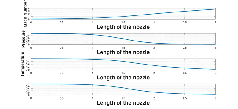
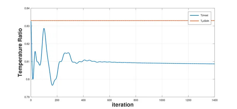
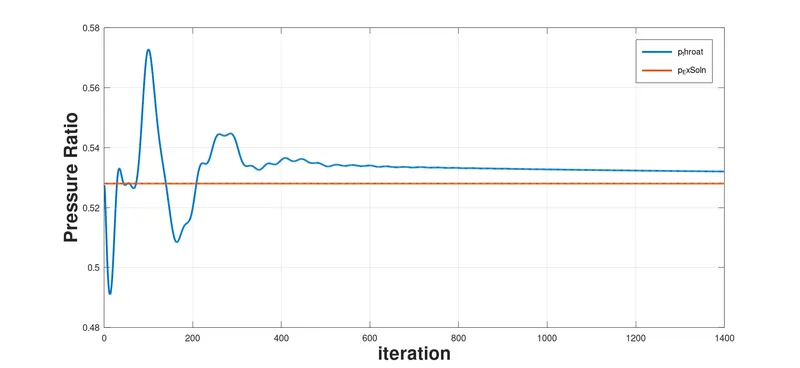
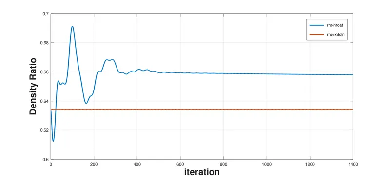
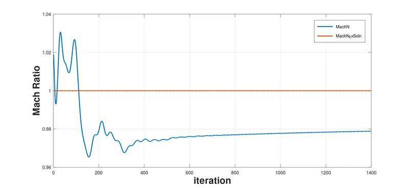
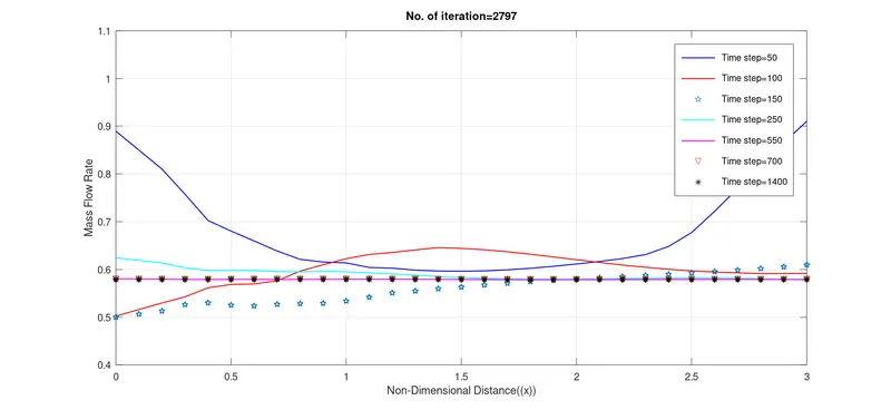
Results for Non-Conservative Form -

Data Inference-

n=31
terms	Eact_Soln	Conservative	Non Conservative
Density	0.634	0.6517	0.63866
Temperature	0.833	0.8407	0.83645
Pressure	0.528	0.5479	0.53421
Mach Number	1	0.9793	0.99939
Mass Flow Rate	0.5792	0.5838	0.5852
n=61
Density	0.634	0.639	0.63766
Temperature	0.833	0.8356	0.83544
Pressure	0.528	0.5339	0.53273
Mach Number	1	0.9979	0.99978
Mass Flow Rate	0.5792	0.5827	0.5828
n=121
Density	0.634	0.63725	0.63171
Temperature	0.833	0.83371	0.83231
Pressure	0.528	0.53137	0.52578
Mach Number	1	0.99823	0.98763
Mass Flow Rate	0.5792	0.5806	0.5808

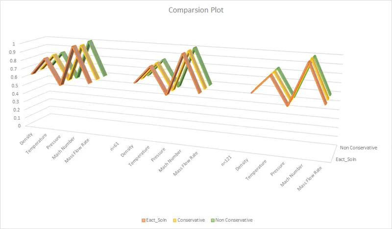
Conculsion-

• Non-Conservative form has less computational time but that merely depends upon the numerical algorithms.
• Also they are more accurate results for primitive variables.
• Whereas in case of Conservative form they yield to better mass flow distribution.
• Here conservative show more accurate results for flux terms.
• If we compare the amount of calculation effort taken by both forms for achieving the soln, then Conservative form requires marginally more work.
• This happens due to the decoding of the primitive variables from Flux and Source terms comparatively Non-Conservative form does not require such decode.