Week 4 - CHT Analysis on Exhaust port

Objective :- CHT Analysis on Exhaust port

Conjugate heat transfer (CHT) :- analysis involves the simulation of heat transfer between solid and fluid domains by exchanging thermal energy at the interfaces between them.The CHT approach has an advantage over FE thermal analysis in that wall heat transfer coefficients and their local variations on surfaces are directly calculated within the model rather than based on simplified empirical calculations. The CHT approach therefore has benefits for those applications where heat transfer is either non-uniform or difficult to calculate empirically.

Application - CHT methods have become a more powerful tool for modeling and investigating nature phenomena and engineering systems in different areas ranging from aerospace and nuclear reactore to thermal goods treatment and food processing from complex procedures in medicine to atmosphere/ocean thermal interaction in meteorology, and from relatively simple units to multistage, nonlinear processes.

The most common in CFD simulation are of heat exchangers, cooling of electronic equipment, and general-purpose cooling and heating systems.

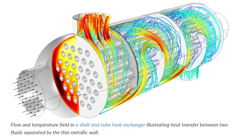
Geometry :-

Meshing :-

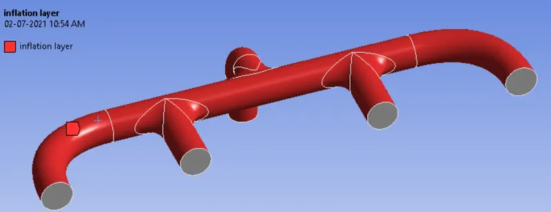
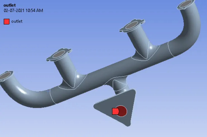
Naming selected boundaries/faces -

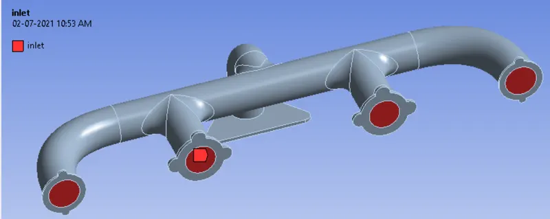
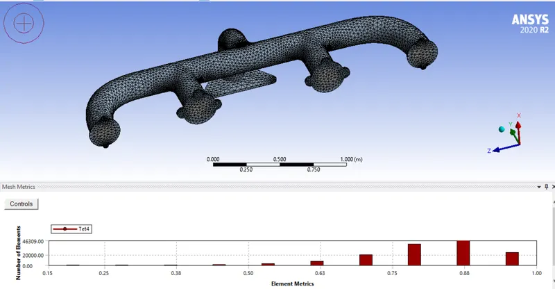
Base line (default) mesh -

Setup :

• Pressure-based solver is used, as Mach no. <0.3 & no major compressions of fuid involed. Here as we are intersted in final Temperature distribution, so steady state analysis is performed.
• Energy Equation turned on.
• K-omega SST viscous model is wall function is used to solve the flow problem, because our focus in on physcis/energy transfer involved at wall or solid-fluid interfernce region.
• Cell Zone : Fluid = Air ; Solid = Aluminum
• Boundary condition -

Inlet Velocity-inlet = 5m/s

Outlet pressure-outlet = 0pa

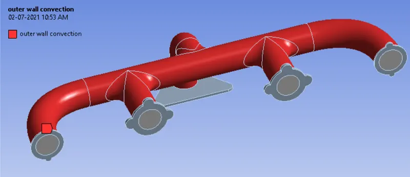
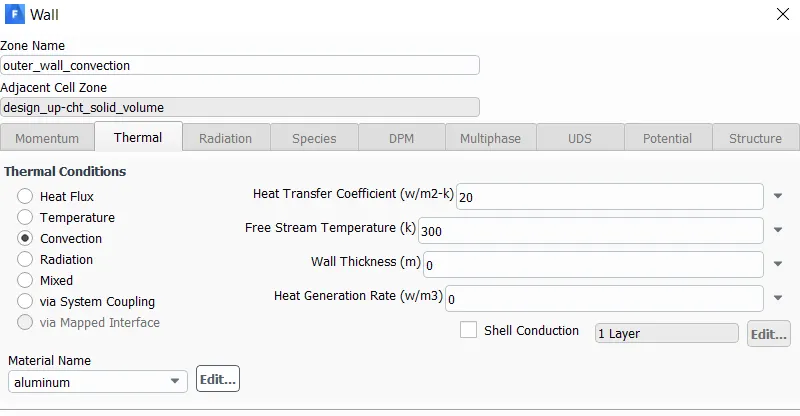
Convection BC : In this aprroach we need not to mesh surrounding fluid(air) domian, where we only need to apply convective BC to external wall in contact with surrounding, thus mesh count will be less & calculations will much more stable. The natural external convection phenomenon can be fulfilled/replicated by providing the Heat transfer co-efficient in the BC rather than fixed temperature, CFD code then calculates based on Newton's Laws of cooling.
By specifying Exteranal Heat transfer co-efficient we providing or quatifying the external (wind) condition , thus how effective heat transfer.

Outer wall convection = 20W/m2-k (constant, with some nusselt correlation this value was derived)

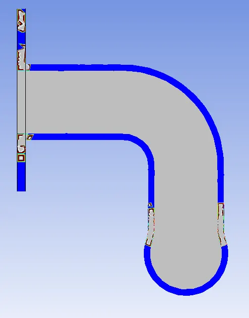
Pipe Flange parts (highlighted body in below) = Adiabatic condition (wall flux = 0)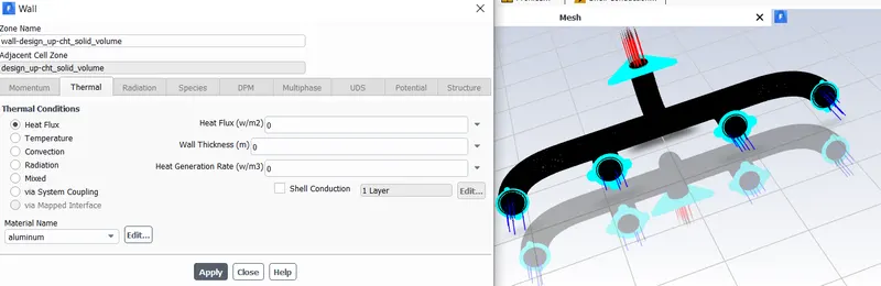

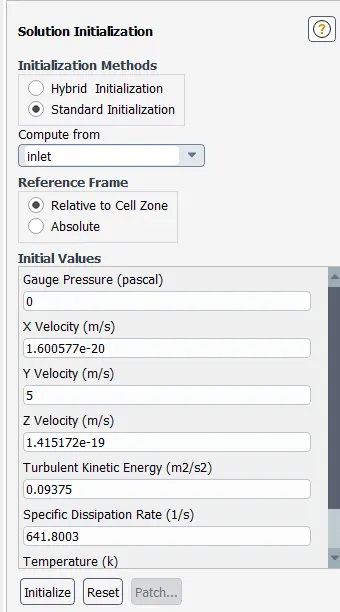
• Standart Intilization computed from Input
• Coupled method by default suggested by Ansys is used for calculation.

Results :

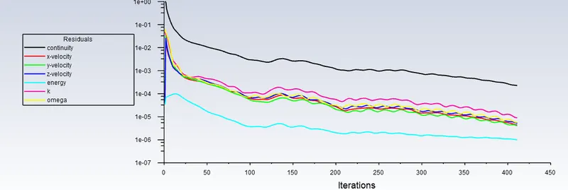
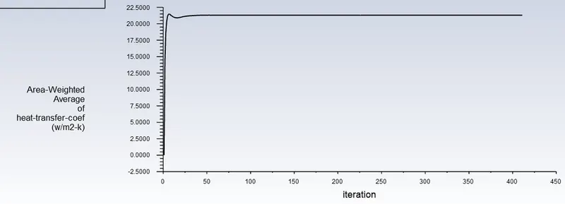
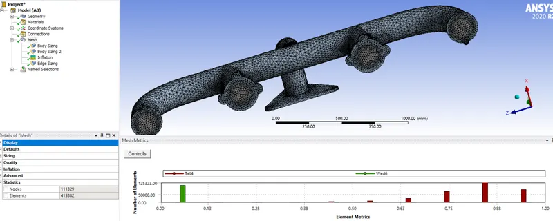
Refined mesh - To obtain accurate results mesh is refined accordingly near wall.

Element sizes

Fluid volume body	Solid volume body	Edge sizing	inflation layers (local)
15mm	50mm	48 nos	8

Maintaining the y+ value according to the K-omega turbulence model :

For heat transfer flow rigimes near wall mesh resolution required thus integrating through viscous sublayer for Y+ should be 0.1 to 5.Here the fluid flowing very close to the wall is dominated by viscous shear in the absensce of turbulent shear.

Y+ = 1 , Using Y+calculator first layer thickness = 0.05610169mm.

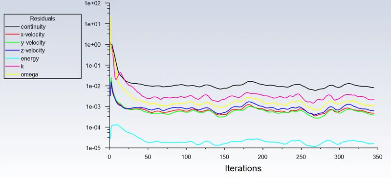
Results -

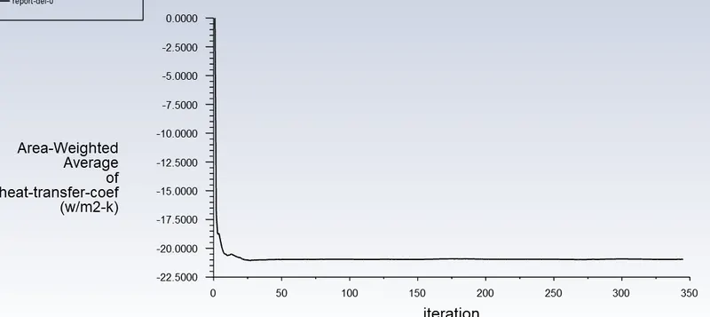
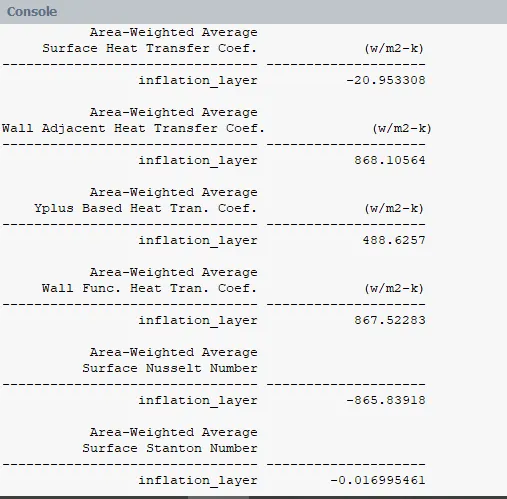
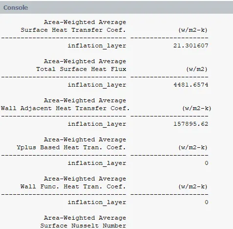
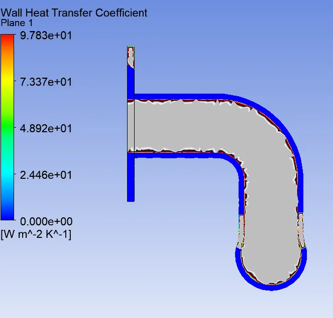
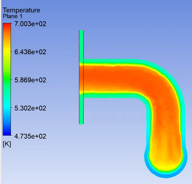
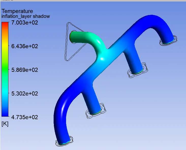
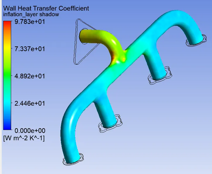
Wall surface Heat Transfer distribution

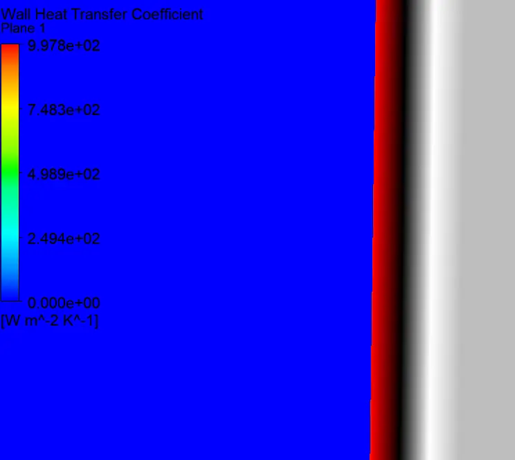
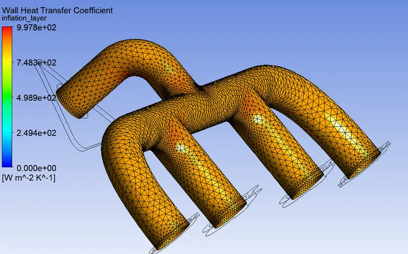
• We can observe that max convective heat transfer is b/w fluid & solid interferace.
• At the solid pipe part c/s the conduction heat transfer is almost constant.

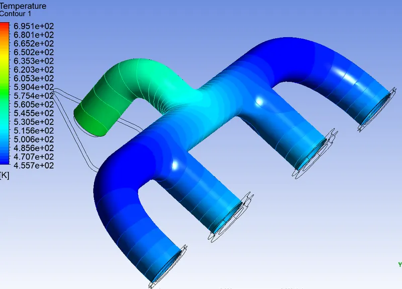
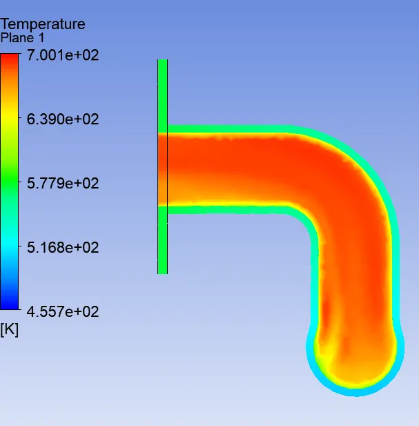
• The temperature distribution inside the pipe will be mostly parabolic involving hot fluids at the centre of pipe.

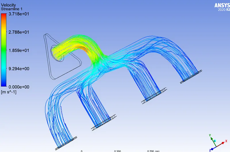
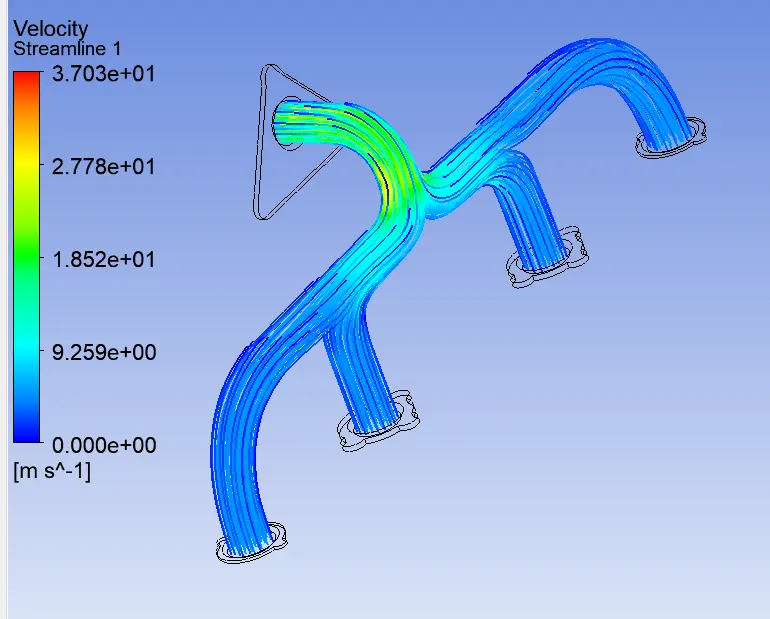
• The velocity at the outlet connected pipe is higher as mass flow rate is high (Mass from 4 inlets causing) thus more heatflux is drawn out through solid pipe at outlet elbow.

Verifying HTC simulation soultion -

Empirical correlation captures the condition outside the pipe and often these corrrelations are pressented as Nuuselt number (h ext is dimensionless)

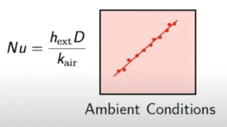
For the given flow Reynolds no =58189.9, which is turbulent. Since the analysis of turbulent flow conditions is a good deal more involved, greater emphasis is placed on determining empirical correlations. A classical expression for computing the local Nusselt number for fully developed (hydrodynamically and thermally) turbulent flow in a smooth circular tube is Dittus-Boelter equation is the preffered version for flow in circular tubes

given by `Nu = 0.023*Re 4/5* Pr1/3`

w.k.t Prandalt no. `Pr = (mu *Cp )/k`

`mu`Dynamic viscosity of fluid (air) = 1.7894e-05 kg/m-s

`Cp` Speacific heat of fluidat constant pressure = 1006.43 j/kg-k

Now , `Pr = (1.7894e-05 * 1006.43 )/0.0242 = 0.7442`

Now , `Nu= 0.023*58189.9 ^ (4/5)* 0.744^(1/3) = 135.1562`

therefore HTC is calculated -

`H (ext) = (Nu * K) /D = (135.15*0.0242)/0.17 = 19.24`

HTC = 19.23 W/m2-k

Devation = Numerical - analystical = 20.95 -19.23 = 8.94%