Challenge

Week 4 - CHT Analysis on Exhaust port

SSuhail Ahmed S21 Jun 2023

CHT ANALYSIS ON EXHAUST PORT

AIM: To stimulate the internal flow for CHT analysis on exhaust port for different cases like coarse mesh and refined mesh.

OBJECTIVE:

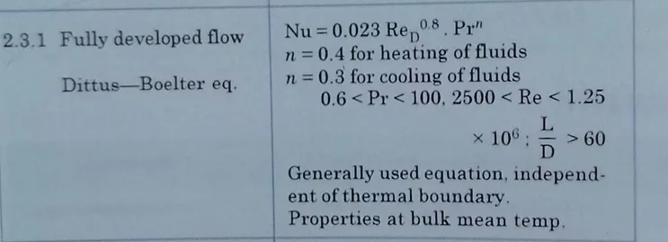
To attain the maximum heat coefficient while comparing analytical and theoretical calculation for CHT analysis on exhaust port.

Expected results: -

Give a brief description of why and where a CHT analysis is used.
Maintain the y+ value according to the turbulence model and justify the results.
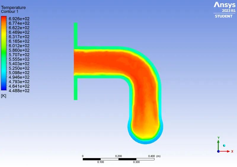
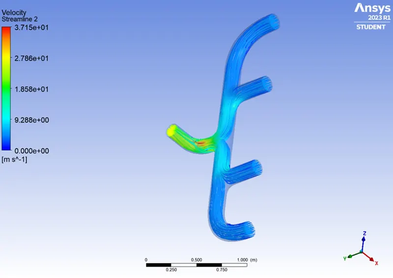
Calculate the wall/surface heat transfer coefficient on the internal solid surface & show the velocity & temperature contours in appropriate areas.
How would you verify if the HTC predictions from the simulations are right? On what factors does the accuracy of the prediction depend on?

INTRODUCTION:

Conjugate heat transfer corresponds with the combination of heat transfer in solids and heat transfer in fluids. In solids, conduction often dominates whereas in fluids, convection usually dominates. Conjugate heat transfer is observed in many situations. For example, heat sinks are optimized to combine heat transfer by conduction in the heat sink with the convection in the surrounding fluid.

Heat Transfer by Solids and Fluids

Heat Transfer in a Solid:

In most cases, heat transfer in solids, if only due to conduction, is described by Fourier’s law defining the conductive heat flux, q, proportional to the temperature gradient: .

For a time-dependent problem, the temperature field in an immobile solid verifies the following form of the heat equation:

Heat Transfer in a Fluid

Due to the fluid motion, three contributions to the heat equation are included:

The transport of fluid implies energy transport too, which appears in the heat equation as the convective contribution. Depending on the thermal properties on the fluid and on the flow regime, either the convective or the conductive heat transfer can dominate.
The viscous effects of the fluid flow produce fluid heating. This term is often neglected, nevertheless, its contribution is noticeable for fast flow in viscous fluids.
As soon as a fluid density is temperature-dependent, a pressure work term contributes to the heat equation. This accounts for the well-known effect that, for example, compressing air produces heat.

Accounting for these contributions, in addition to conduction, results in the following transient heat equation for the temperature field in a fluid:

Conjugate Heat Transfer Applications

Effective Heat Transfer

Efficiently combining heat transfer in fluids and solids is the key to designing effective coolers, heaters, or heat exchangers.

The fluid usually plays the role of energy carrier on large distances. Forced convection is the most common way to achieve high heat transfer rate. In some applications, the performances are further improved by combining convection with phase change (for example liquid water to vapor phase change).

Even so, solids are also needed, in particular to separate fluids in a heat exchanger so that fluids exchange energy without being mixed.

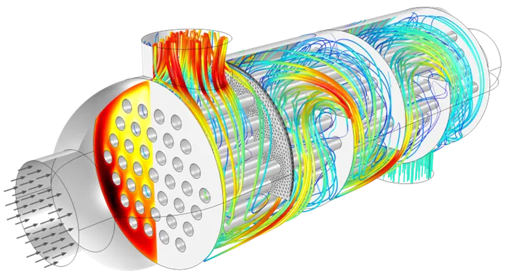
Flow and temperature field in a shell and tube heat exchanger illustrating heat transfer between two fluids separated by the thin metallic wall.

Heat sinks are usually made of metal with high thermal conductivity (e.g., copper or aluminium). They dissipate heat by increasing the exchange area between the solid part and the surrounding fluid.

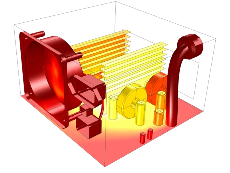
Two aluminium fins are used to increase the exchange area between the flow and the electronic components.

Energy Savings

Heat transfer in fluids and solids can also be combined to minimize heat losses in various devices. Because most gases (especially at low pressure) have small thermal conductivities, they can be used as thermal insulators… provided they are not in motion. In many situations, gas is preferred to other material due to its low weight. In any case, it is important to limit the heat transfer by convection, by reducing the natural convection effects. Judicious positioning of walls and use of small cavities helps to control the natural convection. Applied at the micro scale, the principle leads to the insulation foam concept where tiny cavities of air (bubbles) are trapped in the foam material (e.g., polyurethane), which combines high insulation performances with light weight.

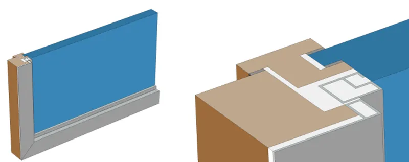
Window cross section (left) and zoom-in on the window frame (right).

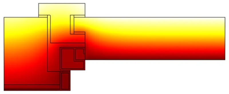
Temperature profile in a window frame and glazing cross section from ISO 10077-2:2012 (thermal performance).

Fluid and Solid Interactions

Fluid/Solid Interface

The temperature field and the heat flux are continuous at the fluid/solid interface. However, the temperature field can rapidly vary in a fluid in motion: close to the solid, the fluid temperature is close to the solid temperature, and far from the interface, the fluid temperature is close to the inlet or ambient fluid temperature. The distance where the fluid temperature varies from the solid temperature to the fluid bulk temperature is called the thermal boundary layer. The thermal boundary layer size and the momentum boundary layer relative size is reflected by the Prandtl number : for the Prandtl number to equal 1, thermal and momentum boundary layer thicknesses need to be the same. A thicker momentum layer would result in a Prandtl number larger than 1. Conversely, a Prandtl number smaller than 1 would indicate that the momentum boundary layer is thinner than the thermal boundary layer. The Prandtl number for air at atmospheric pressure and at 20°C is 0.7. That is because for air, the momentum and thermal boundary layer have similar size, while the momentum boundary layer is slightly thinner than the thermal boundary layer. For water at 20°C, the Prandtl number is about 7. So, in water, the temperature changes close to a wall are sharper than the velocity change.

Normalized temperature (red) and velocity (blue) profile for natural convection of air close to a cold solid wall.

Natural Convection

The natural convection regime corresponds to configurations where the flow is driven by buoyancy effects. Depending on the expected thermal performance, the natural convection can be beneficial (e.g., cooling application) or negative (e.g., natural convection in insulation layer).

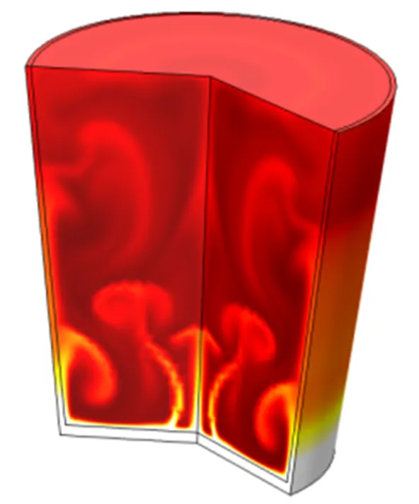
Temperature profile induced by natural convection in a glass of water in contact with a hot surface.

Forced Convection

The forced convection regime corresponds to configurations where the flow is driven by external phenomena (e.g., wind) or devices (e.g., fans, pumps) that dominate buoyancy effects.

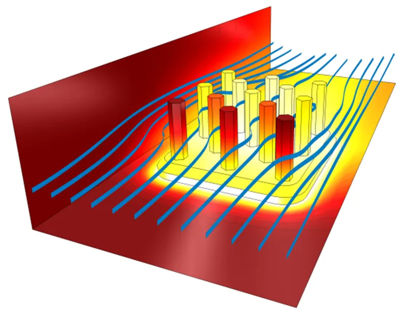
Streamlines and temperature profile around a heat sink cooling by forced convection.

Steps involved in analysis:

Pre-processing
Solving
Post-processing

CASE 1:

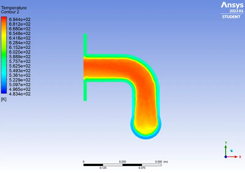
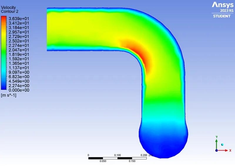
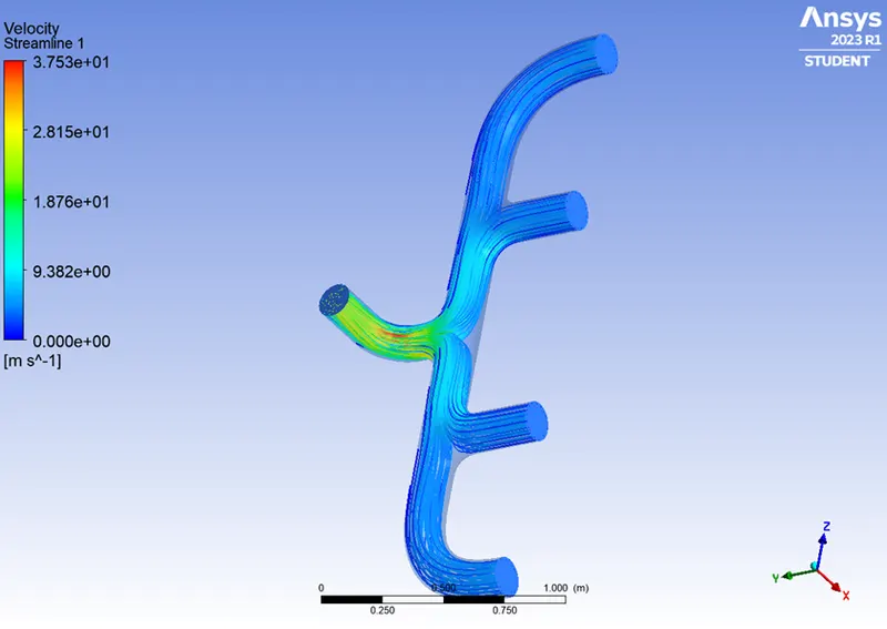
Simulate the flow with the steady state solver with inlet velocity of 5m/s and inlet temperature 700k with this model having coarse mesh.

Pre-processing:

From the analysis system toolbox open the Fluid Flow (Fluent)

In Geometry open the spaceclaim for the 2D designing of the model.

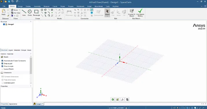
Geometry of the model is imported.

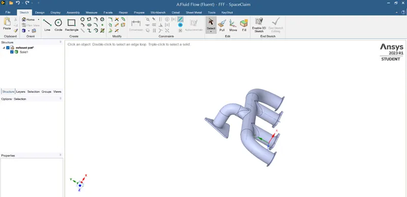
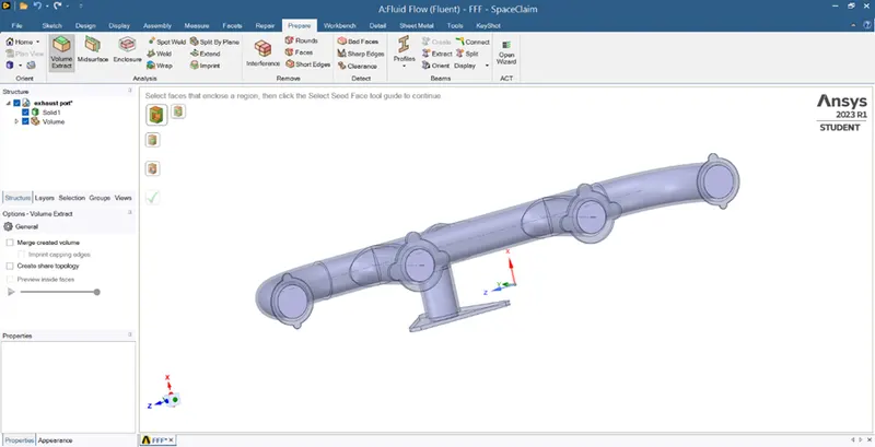
Extract the volume for the internal flow analysis on exhaust port.

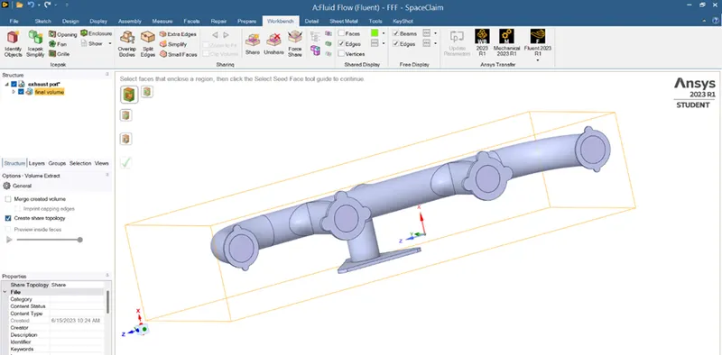
Move the fluid and solid volume into new component as final volume.

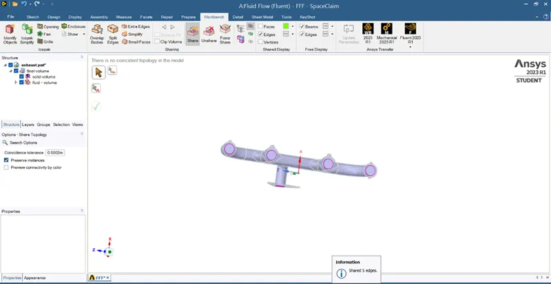
Then share topology of the fluid and solid volume for exact arrangement of mesh.

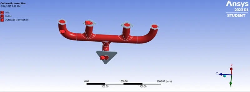
Close the spaceclaim and go to mesh. Create the named selection to the model.

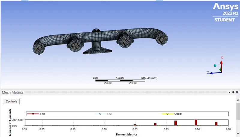
The default mesh is generated, and mesh metric is around 21%

Solving:
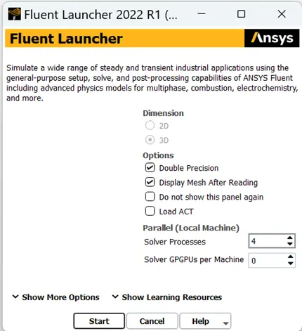
Open the setup for applying the boundary condition for the fluid flow solution.

Setup	LAMINAR
Solver time	Steady state
Solver type	Density Based
Viscous Model	LAMINAR
Material	Air o Density- 1.225kg/m³ o Viscosity - 1.7894e-05 Pa s Aluminium o Density- 2719 kg/m³ o K - 202.4 w/m k
Boundary Condition	· Inlet o Velocity- 5m/s o Temp – 700k · Outlet-wall convection o CHT – 20 w/m²k · Outlet o Pressure Outlet · Fluid volume o Adiabatic [ heat flux – 0w/m²]

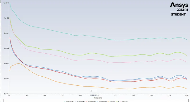
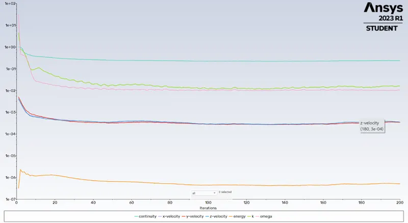
Scaled residual plots.

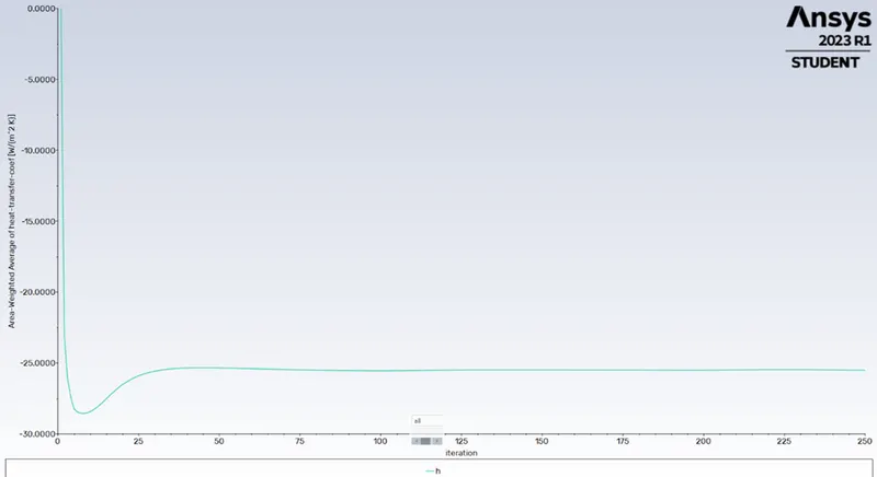
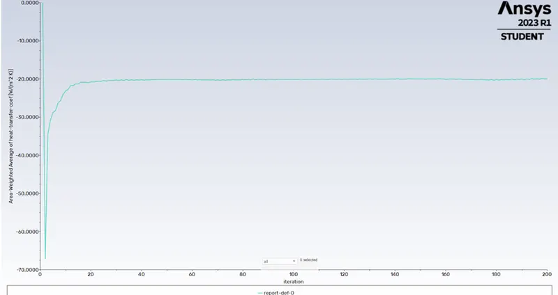
Heat transfer coefficient plot.

Post-processing:
Temperature contour:

Velocity contour:

Velocity streamline:

CASE 2:

Simulate the flow with the steady state solver with inlet velocity of 5m/s and inlet temperature 700k, with this model having refined mesh.

Pre-processing:

From the analysis system toolbox open the Fluid Flow (Fluent)

In Geometry open the spaceclaim for the 2D designing of the model.

Geometry of the model is imported.

Extract the volume for the internal flow analysis on exhaust port.

Move the fluid and solid volume into new component as final volume.

Then share topology of the fluid and solid volume for exact arrangement of mesh.

Close the spaceclaim and go to mesh. Create the named selection to the model.

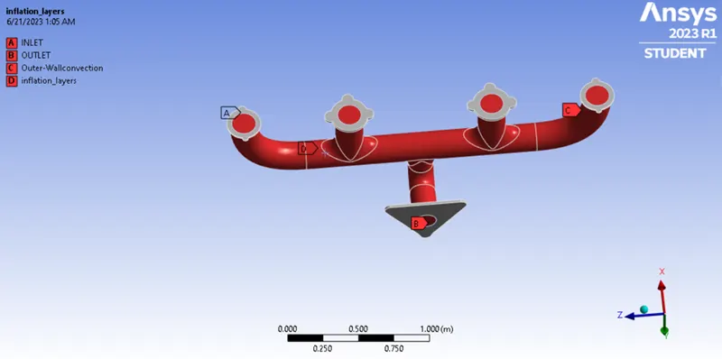
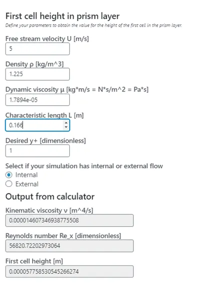
Calculate the first layer thickness using volupe calculator.

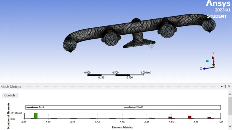
The refined mesh is generated, and the mesh matric is around 6%

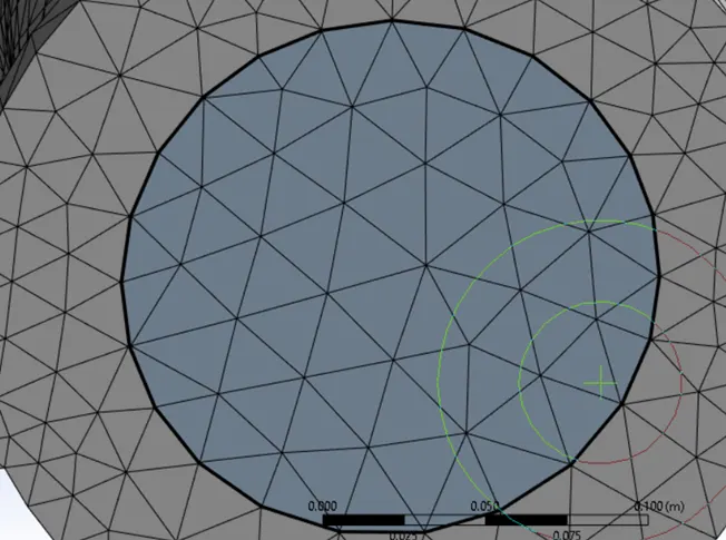
The inflation up to 5 layers is given around the fluid volume.

Solving:
Open the setup for applying the boundary condition for the fluid flow solution.

Setup	LAMINAR
Solver time	Steady state
Solver type	Density Based
Viscous Model	LAMINAR
Material	Air o Density- 1.225kg/m³ o Viscosity - 1.7894e-05 Pa s Aluminium o Density- 2719 kg/m³ o K - 202.4 w/m k
Boundary Condition	· Inlet o Velocity- 5m/s o Temp – 700k · Outlet-wall convection o CHT – 20 w/m²k · Outlet o Pressure Outlet · Fluid volume o Adiabatic [ heat flux – 0w/m²]

Refined mesh: 1 (50mm)

Scaled residual plots.

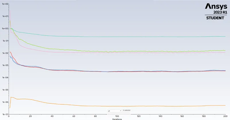
Heat transfer coefficient plot.

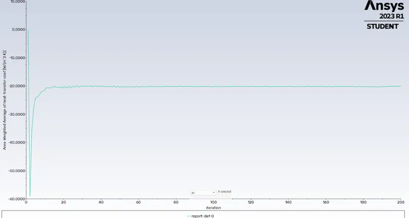
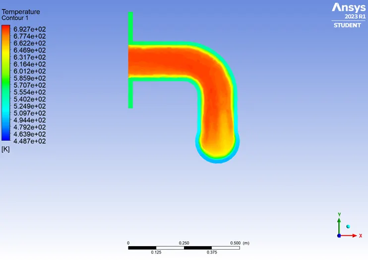
Post-processing:
Temperature contour:

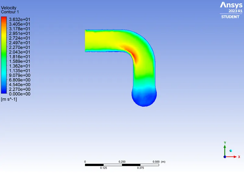
Velocity contour:

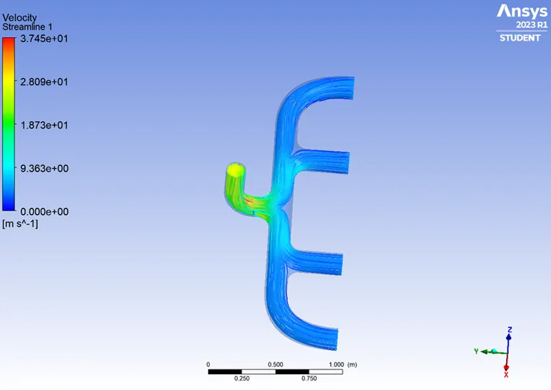
Velocity streamline:

Refined mesh: 2 (10mm)

Scaled residual plots.

Heat transfer coefficient plot.

Post-processing:
Temperature contour:

Velocity contour:

Velocity streamline:

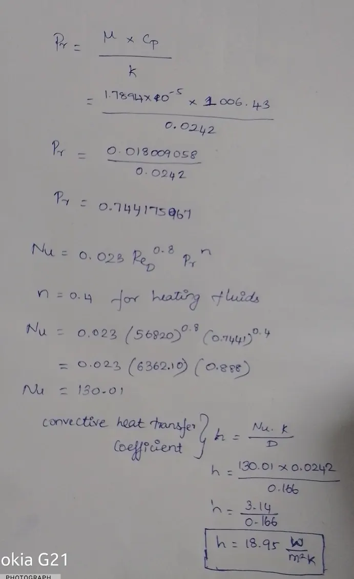
Analytical solution:

Comparison table:

S. No	Mesh sizing	Analytical solution of surface heat transfer coefficient (w/m²k)	Numerical solution of surface heat transfer coefficient (w/m²k)
1	Coarse mesh(0.15mm)	18.95	25.05
2	Refined mesh(0.05mm)		20.09
3	Refined mesh(0.01mm)		19.94

Conclusion:

From the grid independence study results, I conclude that refining mesh size increases the accuracy of the stimulation results.
For the internal flow analysis, k-omega is better than k-epsilon Reynold’s number solver.
Due to multiple inlets & single outlet, the temperature and velocity is high at outlet.

Reference Paper

https://www.researchgate.net/publication/283020042_Simulation_of_Conjugate_Heat_Transfer_CHT_Between_Engine_Head_and_Cooling_Medium_of_Diesel_Engine
https://www.ijeat.org/wp-content/uploads/papers/v6i5/E5007066517.pdf
https://www.academia.edu/65031826/An_Automated_Workflow_for_Efficient_Conjugate_Heat_Transfer_Analysis_of_a_Diesel_Engine