Week 4 - CHT Analysis on Exhaust port
CONJUGATE HEAT TRANSFER ANALYSIS ON EXHAUST PORT
Aim
To simulate the conjugate heat transfer analysis on exhaust port using ANSYS Fluent.
Objectives
- Give a brief description of why and where a CHT analysis is used.
- Maintain the y+ value according to the turbulence model and justify the results.
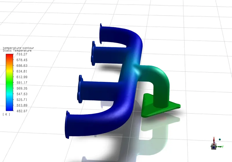
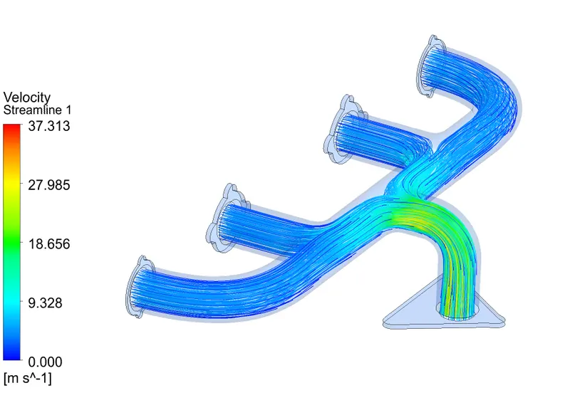
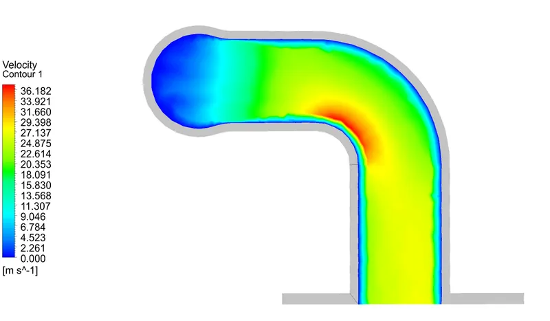
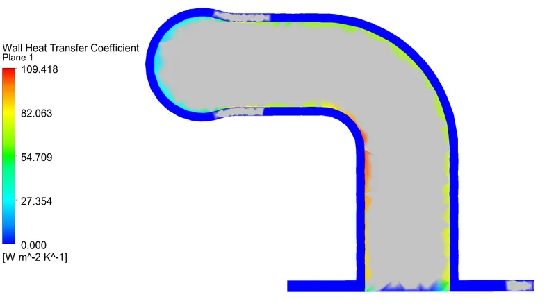
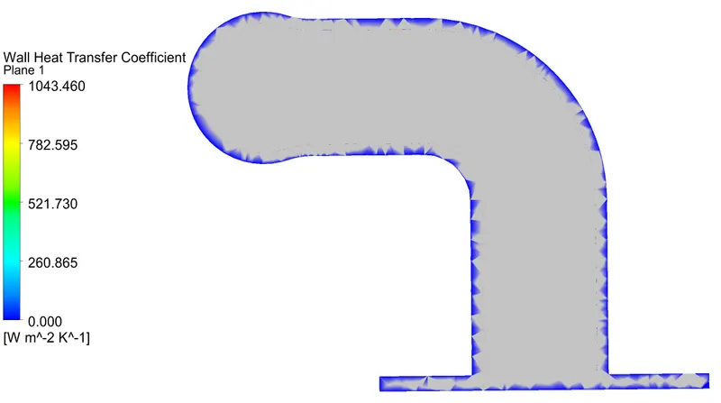
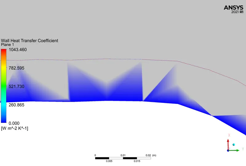
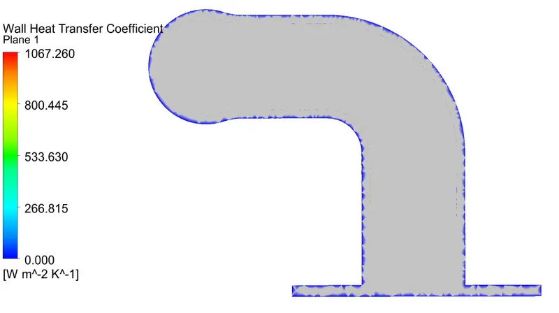
- Calculate the wall/surface heat transfer coefficient on the internal solid surface & show the velocity & temperature contours in appropriate areas.
- How would you verify if the HTC predictions from the simulations are right? On what factors does the accuracy of the prediction depend on?
Introduction
- The term "conjugate heat transfer" refers to the blending of fluid and solid heat transfer. While convection often predominates in fluids, conduction frequently predominates in solids. Numerous scenarios show conjugate heat transfer, for instance, heat sinks are designed to combine fluid convection with heat transfer by conduction within the heat sink.
Heat Transfer in a Solid
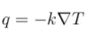
- In the majority of circumstances, Fourier's rule, which states that the conductive heat flow, q, is proportional to the temperature gradient, describes how heat transfer in solids, even if it solely occurs due to conduction:
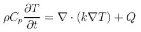
- The temperature field in an immovable solid validates the heat equation in the following form for a time-dependent problem:
Heat Transfer in a Fluid
Three contributions to the heat equation are made because of fluid motion:
- The movement of fluid also involves the movement of energy, which is represented by the convective contribution in the heat equation. Either convective heat transfer or conductive heat transfer may predominate, depending on the thermal characteristics of the fluid and the flow regime.
- Fluid heating is a result of the viscous effects of the fluid flow. Although this concept is frequently disregarded, it contributes significantly to rapid flow in viscous fluids.
- When a fluid's density changes with temperature, a pressure work component enters the heat equation. This explains the well-known phenomenon that, for instance, compressing air generates heat.
- The transient heat equation for the temperature field in a fluid yields the following findings after taking these contributions into account in addition to conduction:

Conjugate Heat Transfer Applications
- The secret to creating efficient coolers, heaters, or heat exchangers is effectively mixing heat transfer in fluids and solids.
- On long distances, fluid often serves as the energy transporter. The most popular method for achieving a high heat transfer rate is forced convection. Combining convection with phase change (such as liquid water to vapour phase transition) might enhance performance in specific applications.
- Solids are still necessary, though, particularly to separate the fluids in a heat exchanger so that they can exchange energy without mixing.
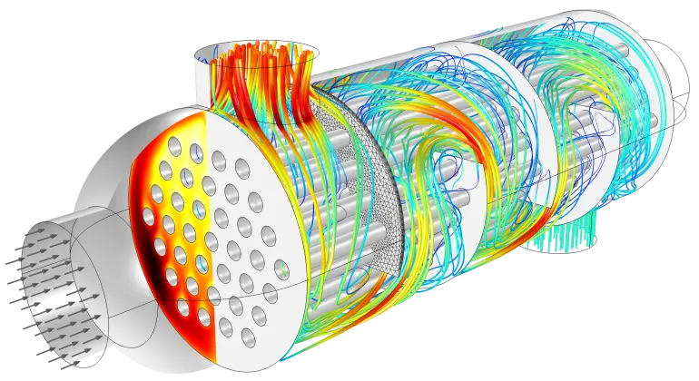
- Heat transmission between two fluids separated by a thin metallic wall is illustrated by the flow and temperature field in a shell and tube heat exchanger.
- Typically, heat sinks are built of high thermal conductivity metals like copper or aluminium. By expanding the region where heat may exchange between the solid component and the surrounding fluid, they disperse heat.
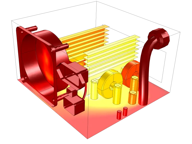
- A power supply unit's temperature field cools as a result of the air flow created by an extractor fan and a perforated grille. The interchange area between the flow and the electrical components is increased using two aluminium fins.
Steps for the Simulation:
- Create the geomentry or load the geomentry
- Discretize the geomentry with adaptable mesh element size
- Apply the material and boundary conditions
- Solve the problem
- Interrupt the results
Problem Setup
Geometry of Exhaust port
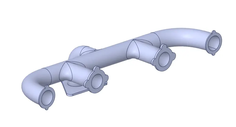
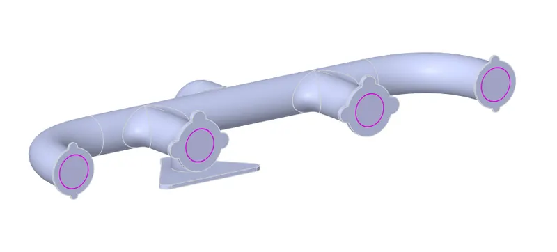
- After importing the exhaust port geometry, extract the fluid volume with the shared topology between fluid volume and solid volume for getting the conformal mesh
Geometry of Exhaust port with shared topology
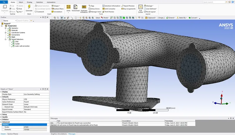
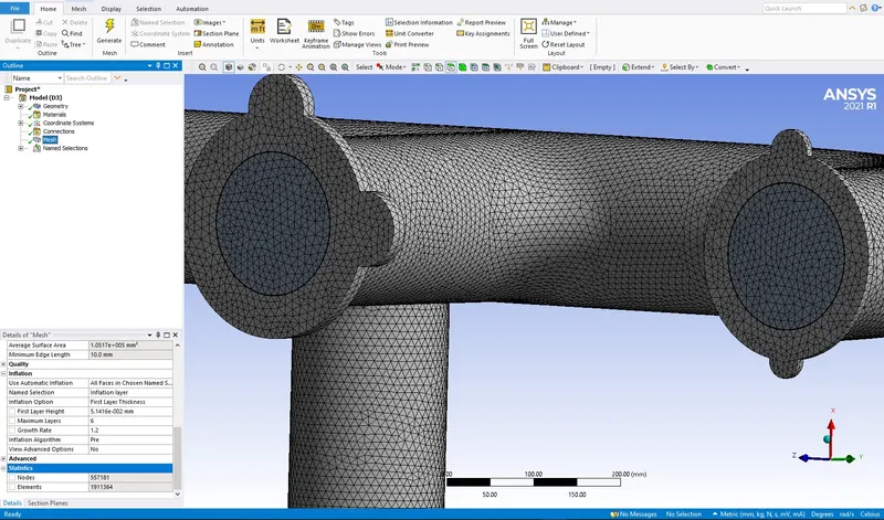
Mesh Setup for finer refinement
It may be deduced that the Y+ value will be in the viscous sub-layer, which is considered to be 1, since the heat transfer coefficient value takes the value of the first cell near the wall. The steps taken to determine the height of the first cell,
`text{Reynold's Number}=\frac{\rho *v*L}{\mu }; text{ L = Characteristics length = inlet diameter}`
`text{ }=\frac{1.225 *5*0.17}{1.7894*10^{-5} }`
`text{ }=58189.89`
`text{Skin friction coefficient}(C_f)=\frac{0.058}{R_e^{0.2}}=\frac{0.058}{58189.89^{0.2}}=0.00646`
`text{Wall shear stress}(tau_w)=0.5*C_f*rho*v^2=0.5*0.00646*1.225*5^2=0.0989Pa`
`text{Frictional velocity}(u_{tau})=(frac{tau_w}{rho})^0.5=(frac{0.0989}{1.225})^0.5=0.2841m/s`
`Y^+=frac{triangley*u_{tau}*rho}{mu}`
For viscous sub-layer Y+ = 1;
`triangley=frac{mu}{u_{tau}*rho}=frac{1.7894*10^{-5}}{0.2841*1.225}=0.0000514162 m=0.0514162 mm`
So, the first layer thickness for the inflation is 0.05141621mm
Solution Setup
- As the given flow's Reynolds number is 58189.89, indicating that it is turbulent. The Nusselt number may be calculated using the Dittus Bolter heat transfer coefficient relation and is theoretically defined as follows,
`Nu_D=0.023*Re_D^{4/5}*Pr^n`
where
`text{Prandtl number}(Pr)={mu*C_p}/k={1.7894*10^{-5}*1006.43}/0.0242=0.744`
n is constant 0.3 heat transfer takes place from fluid to solid
So, `Nu_D=0.023*58189.89^{4/5}*0.744^n=136.483`
`text{Convective heat transfer coefficient}( h)={N_u*k}/D={136.483*0.0242}/0.17=19.429W/{m^2K}`
So, we assume convective heat transfer coefficient at outer wall as 20 `W/{m^2K}` for simulatuion.
Fluent Solver
- Solver type - Pressure-Based
- Energy - On
- Viscous - k-omega ( It was selected because the equation of k-omega predicts the flow near the wall (viscous sub-layer) better than the k-epsilon model
- Material
Fluid - Air
Solid - Aluminium
- Inlet velocity - 5m/s
- Method of solve - Coupled
- Initialization - Hybrid
Results
(i)Baseline Mesh: No of mesh elements - 137555
Mesh
Plots
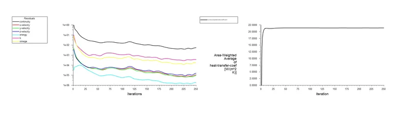
Average Heat Transfer Coefficient value on outer wall surface

Temperature Contour
Streamline Velocity Contour
Velocity Contour
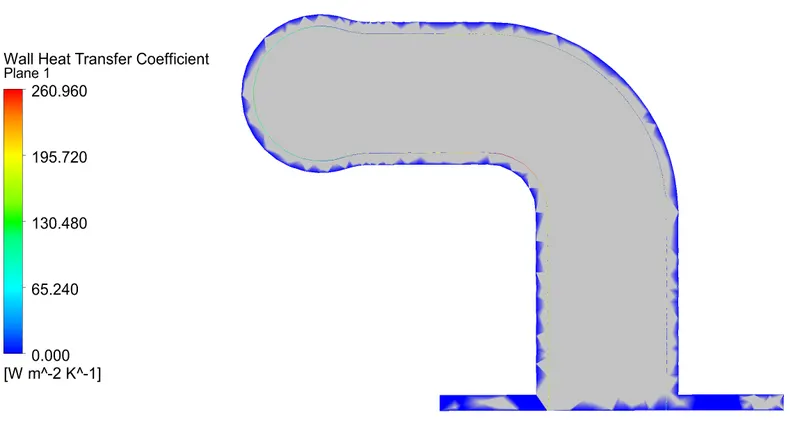
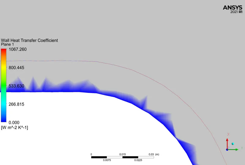
Wall Heat Transfer Coefficient Plot
(ii)No of mesh elements - 317858
Mesh
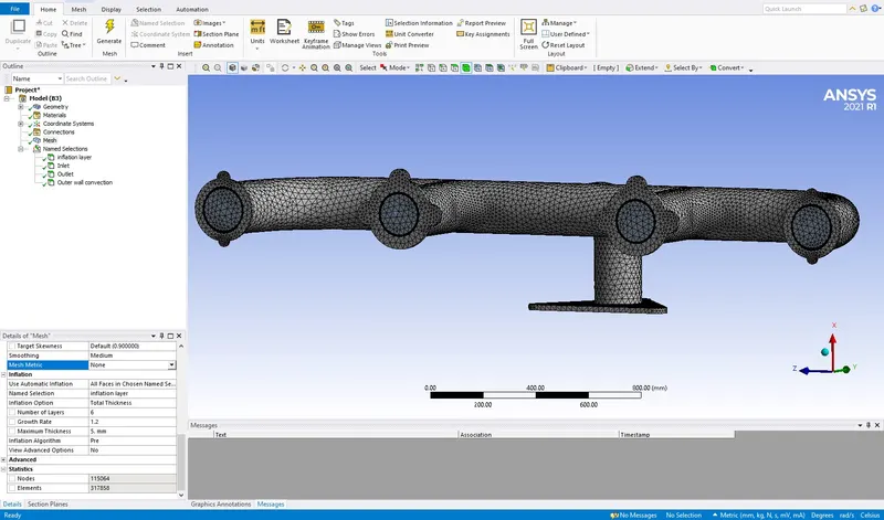
Plots
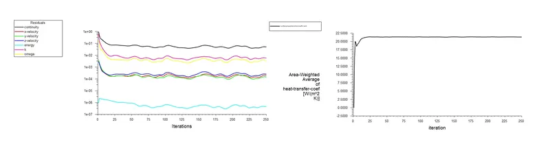
Average Heat Transfer Coefficient value on outer wall surface

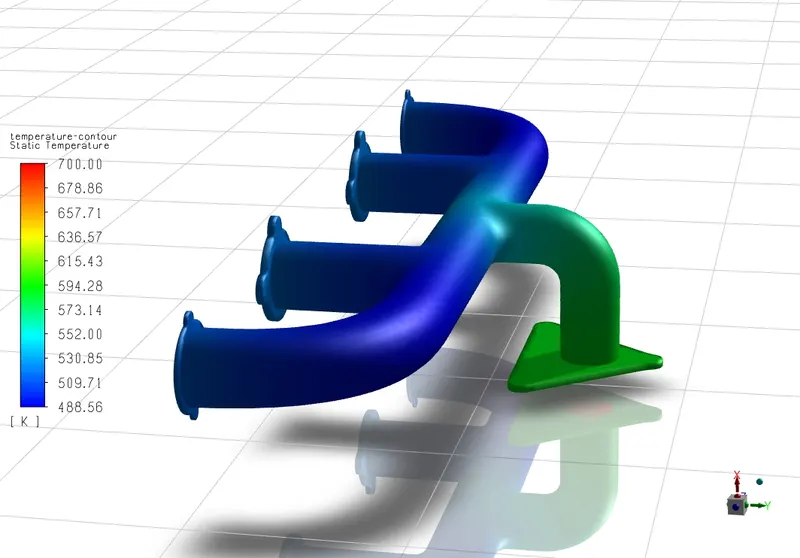
Temperature Contour
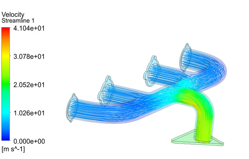
Streamline Velocity Contour
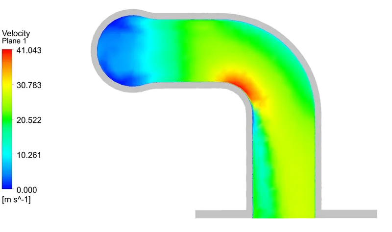
Velocity Contour
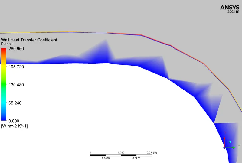
Wall Heat Transfer Coefficient Plot
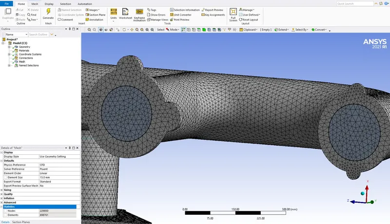
(iii)No of mesh elements - 698761
Mesh
Plots
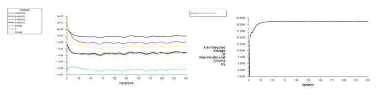
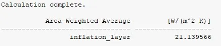
Average Heat Transfer Coefficient value on outer wall surface
Temperature Contour

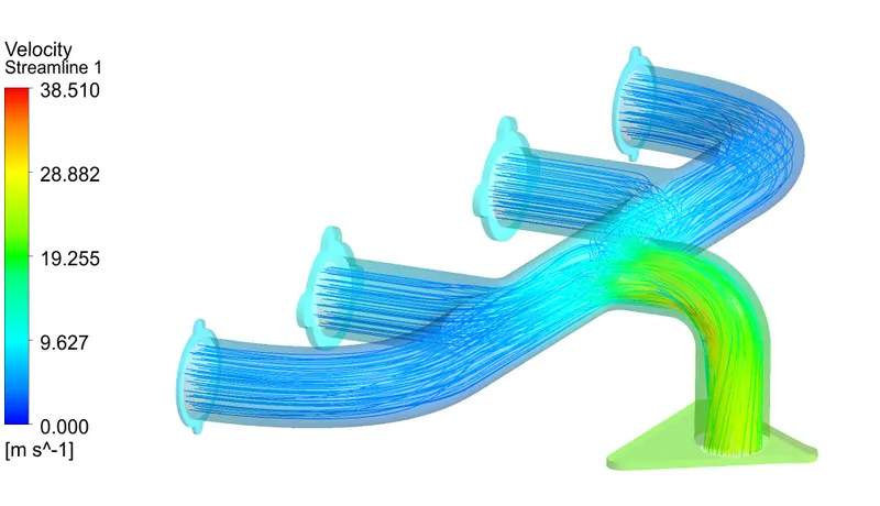
Streamline Velocity Contour
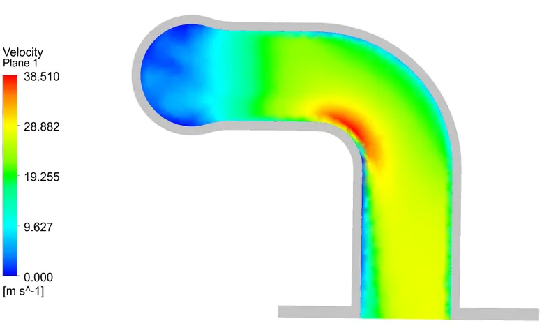
Velocity Contour
Wall Heat Transfer Coefficient Plot
(iv)No of mesh elements - 1911364
Mesh
Plots
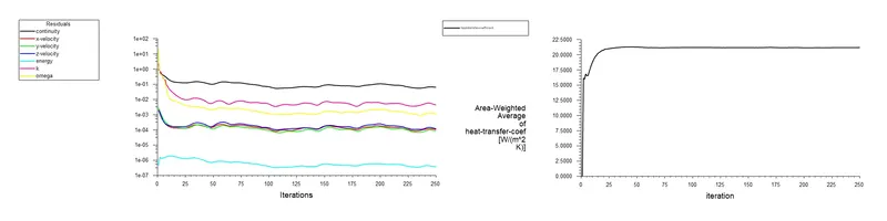
Average Heat Transfer Coefficient value on outer wall surface

Temperature Contour
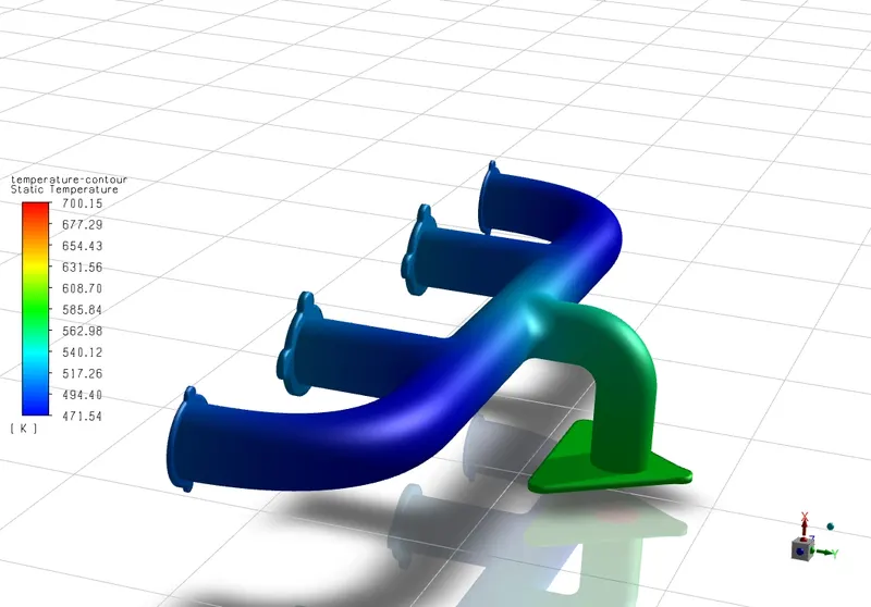
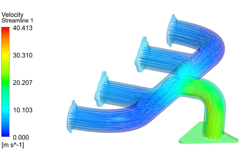
Streamline Velocity Contour
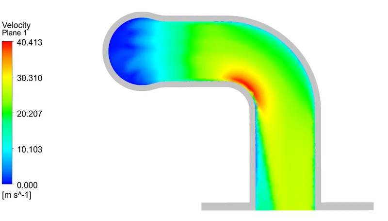
Velocity Contour
Wall Heat Transfer Coefficient Plot
Grid Dependence Test
Sl.No |
No of Mesh Elements |
Surface heat transfer coefficient (Numerical value) `W/{m^2K}` |
Surface heat transfer coefficient (Analytical value) `W/{m^2K}` |
| 1 | 137555 | 21.3651 | |
| 2 | 317858 | 21.3258 | 19.429 |
| 3 | 698761 | 21.1395 | |
| 4 | 1911364 | 21.1765 |
- The key finding is that the surface heat transfer coefficient of outer wall does not change appreciably as mesh fineness increases. Thus, the grid dependency test was successful.
Conclusion
- Using ANSYS-FLUENT, the conjugate heat transfer analysis of the exhaust port was successfully simulated by discretising he model and solve the problem using a pressure-based and coupled scheme solver.
-
We may pick the value of Y+ as viscous sublayer since the heat transfer coefficient value is in the cell next to the wall and based on that we selected the turbulent model as k-omega.
-
The fact that there are four inlets and one outlet explains why the velocity at the outlet is higher than the velocity at the inlet.
- The analytical value of the heat transfer coefficient was 19.429`W/{m^2K}` and the numerical value of the heat transfer coefficient was approximatly 21.1395`W/{m^2K}`
- It was discovered that the numerical heat transfer coefficient values were deviated within 10% of the analytical answer.