Week 5 - Rayleigh Taylor Instability

RAYLEIGH TAYLOR INSTABILITY

Aim

To simulate the Rayleigh Taylor Instability using ANSYS Fluent.

Objectives

• What are some practical CFD models that have been based on the mathematical analysis of Rayleigh Taylor waves.
• Perform the Rayleigh Taylor instability simulation for 2 different mesh sizes with the base mesh being 0.5 mm and compare the results.
• Run one more simulation with water and user-defined material(density = 400 kg/m³, viscosity = 0.001 kg/m-s) for refined mesh.
• Define the Atwood Number. Find out the Atwood number for both the cases and explain how the variation in Atwood number in the above two cases affects the behavior of the instability.

Introduction

Rayleigh Taylor Instability

A phenomenon known as Rayleigh Taylor Instability happens when two fluids with differing densities come in contact and the lighter fluid pushes the heavier fluid because of the density difference. The system attempts to lower its total potential energy in a dynamic process. Taylor instability may happen in a number of circumstances. We give the following examples:

A. Natural occurrences

i) The collapsing core of a huge star toppling on its side.

ii) the development of dual exhaust jets with high brightness in spinning gas clouds in an external gravitational potential.

B. Technology-related uses

Deuterium-tritium fusion target laser implosion.

ii) metal liner electromagnetic implosion, among other things.

Let's quickly review one of these examples. A glass or metal tamper encircles a DT sphere. This tamper is exposed to a powerful laser beam, which accelerates it inward. During the earliest stages of the implosion, the outer surface of the tamper, which is the interface between a heavy fluid (metal) and a light fluid (vaporised metal), is unstable. The pressure of the compressed pellet builds until it is enough to stop the tamper from moving inside, at a compression of the pellet of perhaps 1,000 times its usual density. Taylor instability also characterises this stage of the implosion; in this instance, the DT is pushing the tamper. Despite being so absurdly oversimplified, this illustration of the implosion of a DT pellet nonetheless makes it evident that Taylor instability must be taken into account when assessing pellet performance.

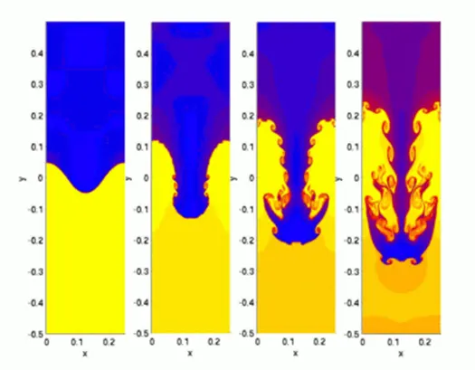
CFD models that have been based on the mathematical analysis of Rayleigh Taylor waves:

• Kelvin–Helmholtz instability
• Plateau–Rayleigh instability
• Richtmyer–Meshkov instability
• Saffman–Taylor instability
• Mushroom cloud
• Salt fingering

From the above list some of them were discussed below,

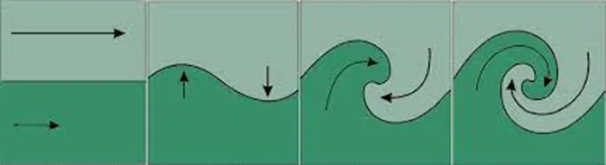
Kelvin-Helmholtz instability

When there is a velocity differential at the interface between two fluids or when there is a velocity shear in a single continuous fluid, this instability frequently develops. The instability constant may be observed as waves on water surfaces, which is a common illustration of how it manifests itself when wind blows over a body of water. In addition to water surfaces like clouds, the Kelvin-Helmholtz instability is also visible in the ocean and the sun's corona, among other natural phenomena. In fluids of varying densities moving at various speeds, the theory predicts the development of instability and change to turbulent flow. This instability develops whenever there is a shear or velocity differential at the fluid interface.

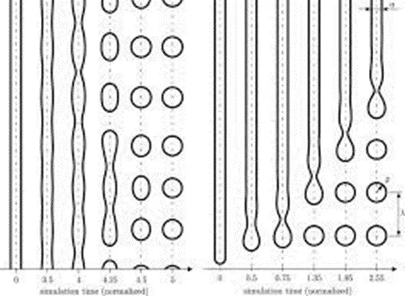
Plateau-Rayleigh instability

A falling stream of fluid breaks up into smaller packets with the same volume but less surface area because of this instability, which is frequently referred to as the Rayleigh instability. It is associated with RTI and belongs to a larger area of fluid dynamics that deals with fluid thread breaking. A specific kind of ink jet technology uses this fluid instability to its advantage by perturbing the liquid jet into a continuous spray of droplets. Liquids have a tendency to have smaller surface areas due to their surface tension, which is what causes the Plateau-Rayleigh instability.

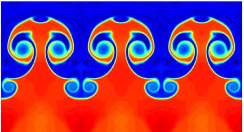
Richtmyer-Meshkov instability

When two fluids with differing densities are impulsively accelerated, this happens. Usually, a shock wave will pass through to do this. Small amplitude disturbances that first increase linearly with time are the beginning stages of the instability's development. After that, a nonlinear regime sets in, where bubbles occur when a light fluid penetrates a heavy fluid and spikes appear when a heavy fluid penetrates a light fluid. The two fluids finally combine as a chaotic regime. This instability may be thought of as the Rayleigh Taylor instability's impulsive-acceleration limit.

Atwood number

In fluid dynamics, the Atwood number (A) is a dimensionless number that is used to examine hydrodynamic instabilities in density stratified flows.

`A={rho_1-rho_2}/{rho_1+rho_2}`

ρ₁ is heavier fluid density

ρ₂ is lighter fluid density

Steps for the Simulation:

• Create the geomentry or load the geomentry
• Discretize the geomentry with adaptable mesh element size
• Apply the material and boundary conditions
• Solve the problem
• Interrupt the results

Problem Setup

Geometry

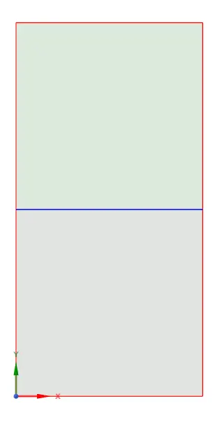
We take into account a straightforward 2D geometry of two squares stacked one on top of the other, each with a length of 0.02 m, and a shared topology for a flawless mesh intersection between the two surfaces.

Fluent Solver

• Solver type - Pressure-Based
• Time - Transient
• Enable Gravity - On Y-axis -9.81 m/s^2
• Multiphase flow - On - Volume of fluid - Set to Implicit and choose Primary Phase and Secondary Phase
• Viscous - laminar
• Material

(i)Fluid - water and Air

(ii)Fluid - water and user-defined material(density = 400 kg/m³, viscosity = 0.001 kg/m-s)

• Method of solve - Coupled
• Initialization - Standard Initialisation and Patch Water as '1' and air as '0'
• Add Contours of Volume fraction of Water and set it to recoed the animation for ever iteration
• Solve it.

Results:

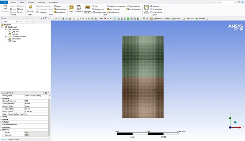
(i)Water and Air: Baseline Mesh - No of mesh elements - 3200

Mesh

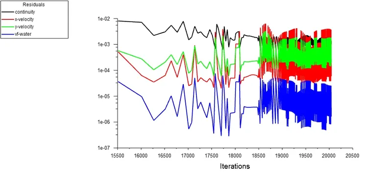
Residuals Plot:

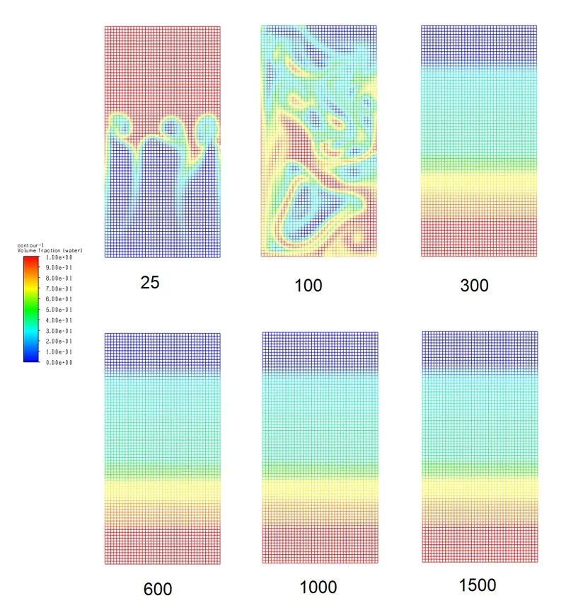
Fluid Instability at different iterations:

Instability Animation link: https://drive.google.com/file/d/1Vuy27PY-VsveQt99j7_369BLyBcfm8pu/view?usp=drivesdk

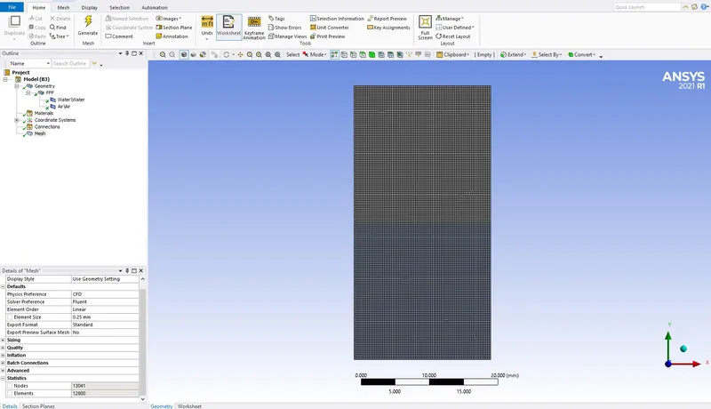
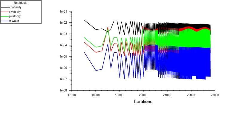
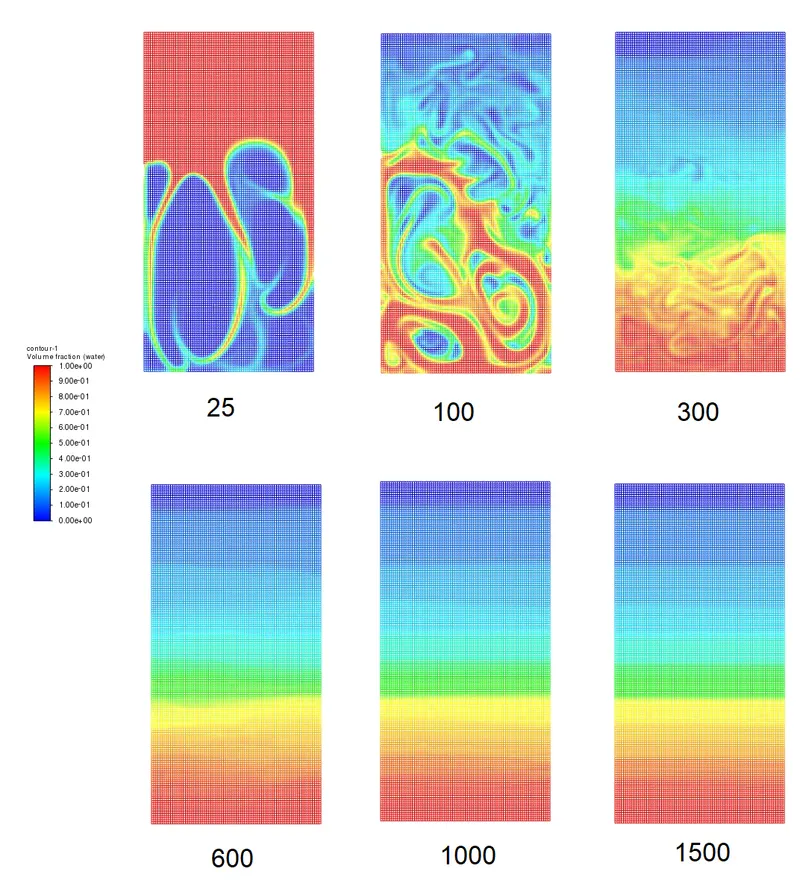
(ii)Water and Air: Fine Mesh - No of mesh elements - 12800

Mesh

Residuals Plot:

Fluid Instability at different iterations:

Instability Animation link: https://drive.google.com/file/d/1KtQsvn3eu5ZSUaf_Bqeq6hDQX9Z_fAkb/view?usp=drivesdk

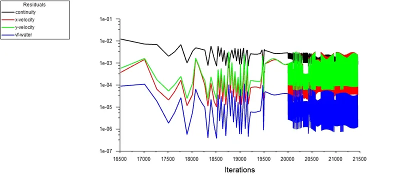
(iii)Water and user defined material: Fine Mesh - No of mesh elements - 12800

Mesh

Residuals Plot:

Fluid Instability at different iterations:

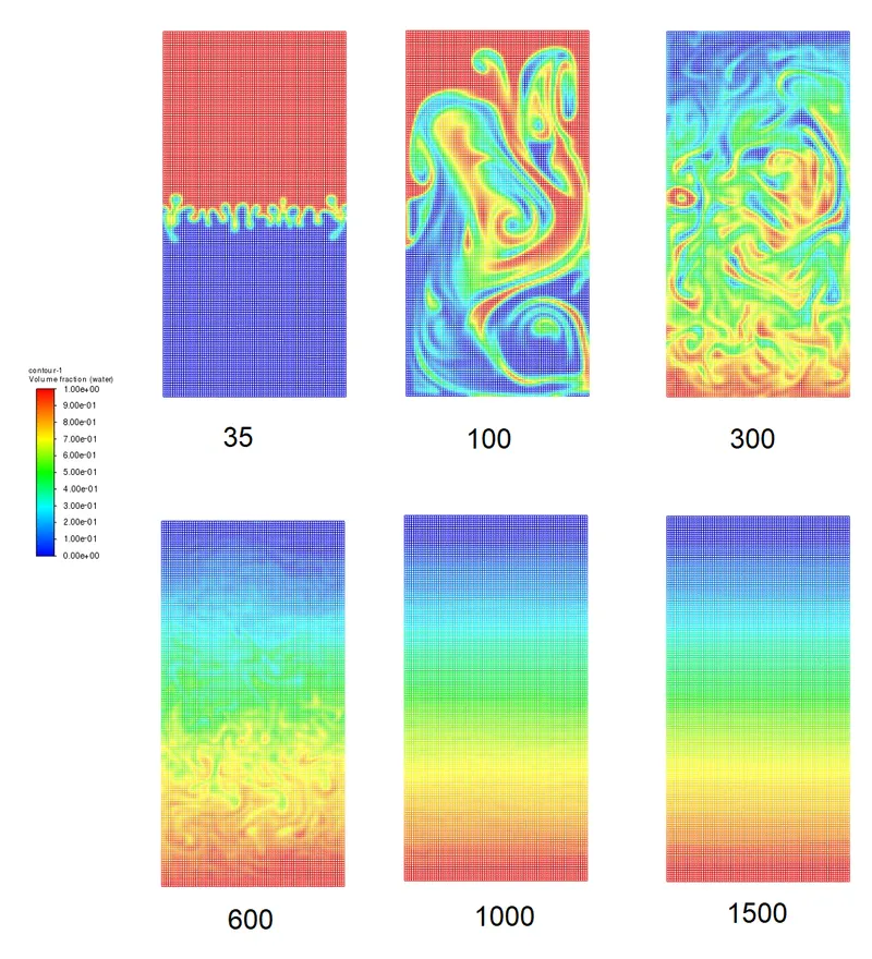
Instability Animation link: https://drive.google.com/file/d/1SmjzFOAcj9Vt_TcqDN3PEj78qez3naTf/view?usp=drivesdk

Calculation of Atwood Number

Case-1: Water and Air

`rho_1=998.2\ {kg} /m^3[text{Water density}]`

`rho_2=1.225\ {kg} /m^3[text{Air density}]`

`A = (998.2-1.225)/(998.2+1.225)=0.998`

Case-2: Water and User defined material

`rho_1=998.2\ {kg} /m^3[text{Water density}]`

`rho_2=400\ {kg} /m^3[text {User defined material density}]`

`A = (998.2-400)/(998.2+400)=0.428`

Rayleigh Taylor's Instability on Atwood number variation:

Linear stability, mushroom head (falling) or bubble (rising) generation, and long term development owing to bubble merging and mixing are the three different stages of Rayleigh Taylor's Instability evolution. When the Atwood number is low, the bubble and mushroom head shape is reasonably symmetrical, and the disturbances or perturbations are linear over a longer time period. In contrast, with big Atwood numbers, the bubble and mushroom head form is less symmetrical, and it happens very quickly and at an increasing pace, resulting in a nonlinear growth rate. On the other side, if there is less of a disparity between the densities, there will be less acceleration and instability. The phase will gradually alter. It will take longer to calm down. In the case of a turbulence model, the splashing effect will be less noticeable, and we may see a nearly symmetrical pattern with an accelerated growth rate.

Reason for Transient state instead of steady state:

We are interested in studying the flow pattern and phase change behaviour of the two fluids at each time step in the Rayleigh Taylor Instability simulation. Since the phase shift in a transient simulation involves time-bound behaviour, a steady state simulation is used since it is a time-independent examination. Every step where a transient simulation is appropriate requires that we keep an eye on the mixing pattern. Simulating in a steady state is only done when the end result is the sole thing we are interested in and blending fluid behaviour is not required. The simulation duration will be shorter here, though.

Conclusion

• It is possible to precisely visualise the Rayleigh Taylor instability of two fluids from the animation video. Additionally, it is found that fine meshing, as opposed to baseline meshing, provides a clearer image of simulation.
• The transient technique is favoured over the steady-state approach because the simulation must capture instabilities that change in an unanticipated way over time.
• The higher the atwood number, the more abrupt the instabilities are and the faster they reach a stable state. Reduce the Atwood Number of Instabilities Take your time and gradually reach a steady condition.