Week 4 - CHT Analysis on Exhaust port

Aim :-

Perform the heat transfer analysis using ANSYS-Fluent software for the given exhaust port problem and use air as the working fluid with velocity of 5 m/s. Consider Inlet and outlet temperature as 700 K and 300 K respectively. Take the wall heat transfer coefficient as 20 W/m².K.

• Give a brief description of why and where a CHT analysis is used.
• Maintain the y+ value according to the turbulence model and justify the results.
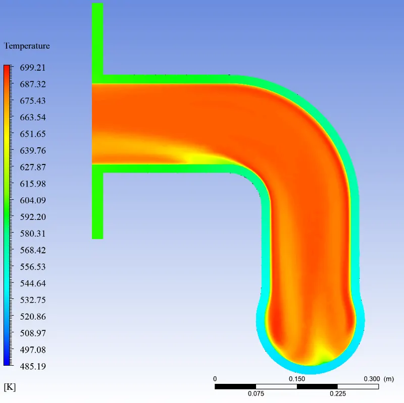
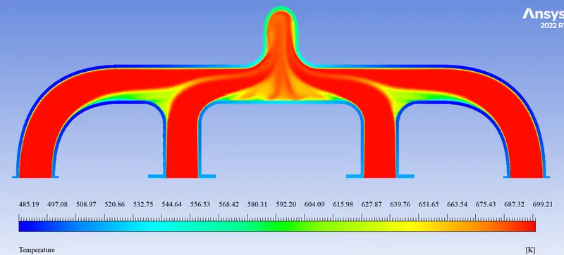
• Calculate the wall/surface heat transfer coefficient on the internal solid surface & show the velocity & temperature contours in appropriate areas.
• How would you verify if the HTC predictions from the simulations are right? On what factors does the accuracy of the prediction depend on?

Introduction :-

CHT Analysis :-

• CHT stands gor Conjugate Heat Transfer.
• The Conjugate Heat Transfer (CHT) analysis type allows for the simulation of heat transfer between solid and fluid domains by exchanging thermal energy at the interfaces between them.

Why a CHT analysis is used ?

The CHT analysis of any given system considers the physical processes and corresponding governing equations involved for the individual subdomains separately and then correlating their solutions by matching the required conditions at the interfaces to get the distribution of temperature and heat flux in a coupled manner thereby eliminating the need of a heat transfer coefficient. A CHT analysis thus offers advantages of monitoring both fluid flow and heat transfer changes as well as real time prediction of wall heat transfer coefficient, temperature and velocity profiles across the domain.

Maintaining Y Plus :-

• Y plus is Non-dimensional distance.
• Y is a distance from wall which is measured as distance from the wall.
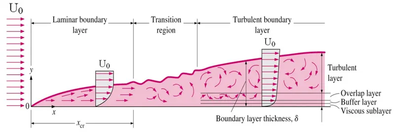
• Here we have to maintain the Y plus value with respect to turbulance model. For Example :-

1. For K omega SST model, the range of Y plus is 0-5.
2. In this case , we have to maintain the Y plus in the range 0-5
3. this will give the correct results.

Procedure :-

• Open Ansys Fluent ans open a fluent module.
• Open geometry Using spaceclaim.
• When opened click on open and select all suported files and now select the exaust port file and open.
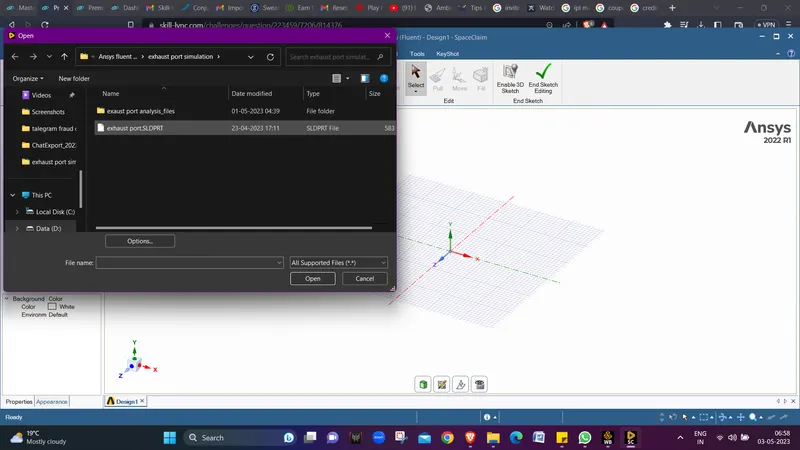
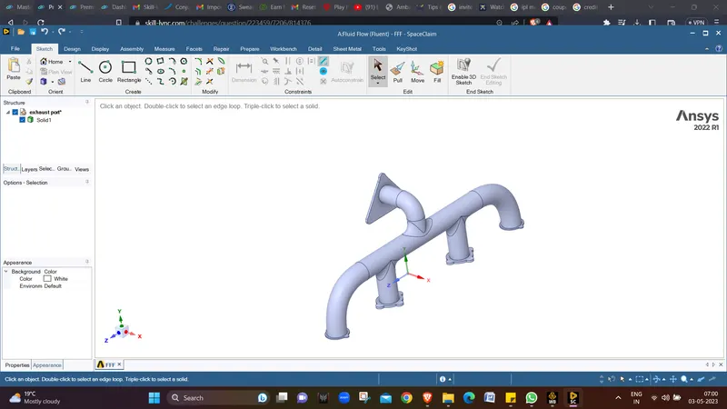
• Now we can see the exaust port model is imported in the workspace.
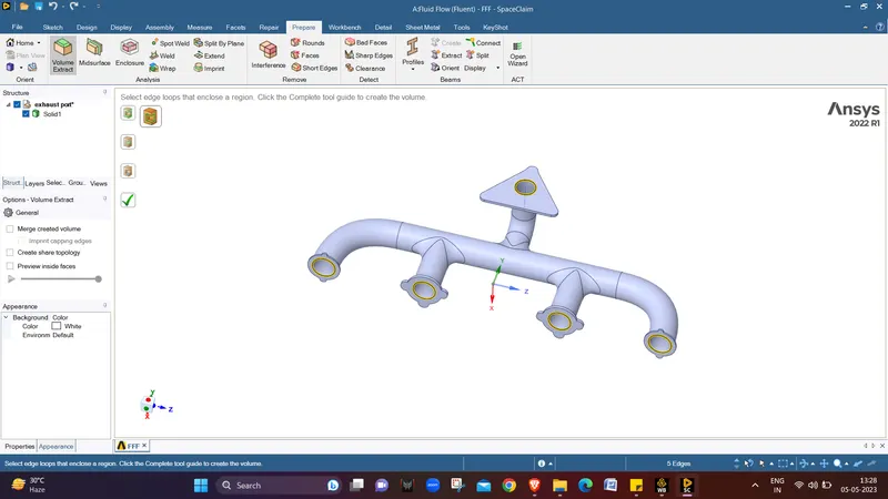
• Now we will extract the fluid volume from the model. Go to Prepare tool bar select volume ectract tool and select edges tool , now select all the edges which need to be used for the volume extraction of fluid, once done select tick mark and the volume will be extracted.
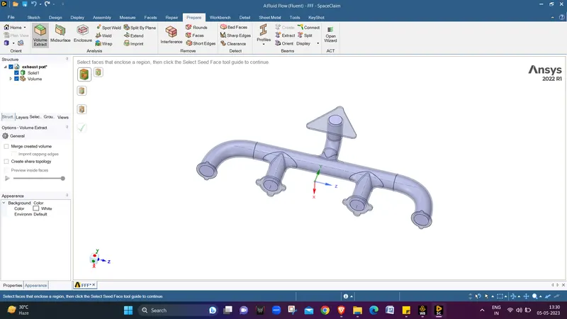
• Now we will go for share topology.
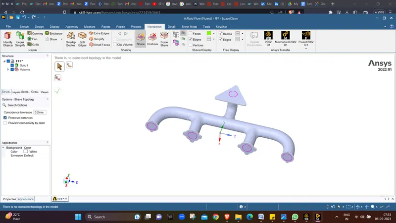
• After enabling the shaertopology we can now close the Geometry window.
• Now we will open meshing module.
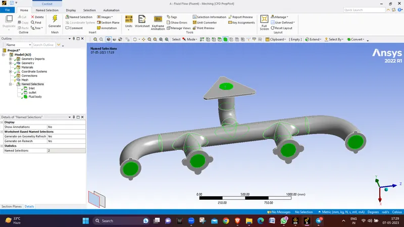
• We will assign name sellection now as
• Inlet of exaust pipes as INLET :-
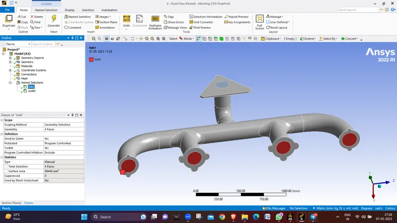
• Exaust oulet pipe as OUTLET :-
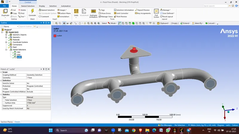
• Fluid volume as FLUID BODY :-
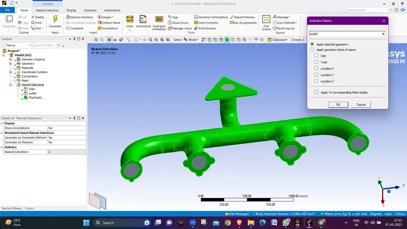
• Outer Body as SOLID :-
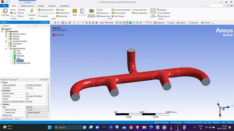
• Fluid outer surface as FLUID WALL :-
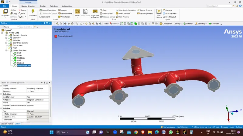
• Outer face of exaust as EXTERNAL PIPE WALL :-
• Now we will proceed towards meshing of this whole exaust port model using some criterias.
• When we apply default mesh size as 150 mm we gett his mesh as a result with number of mesh elements as 138316.
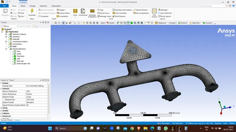
• Now we will give sizing to intenal wall using Sizing tool and using the mesh size as 20 mm.
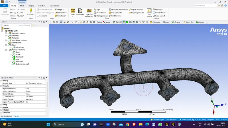
• we can see that we have a finner mesh compared to previous one, Now we will add inflation layers to fluid volume using Y+ calculator to find out first cell height and the growth rate for inflation layers .
• As we know the velocity is 5 m/s and and we will be using y+ value as 1 (as we need really very fine mesh at the fluid wall as we need to find the viscous effect near the pipe wall) and length as 166 mm .
• The first cell height is 0.06 mm and the growth rate is 1.3 with 14 prisum layers .
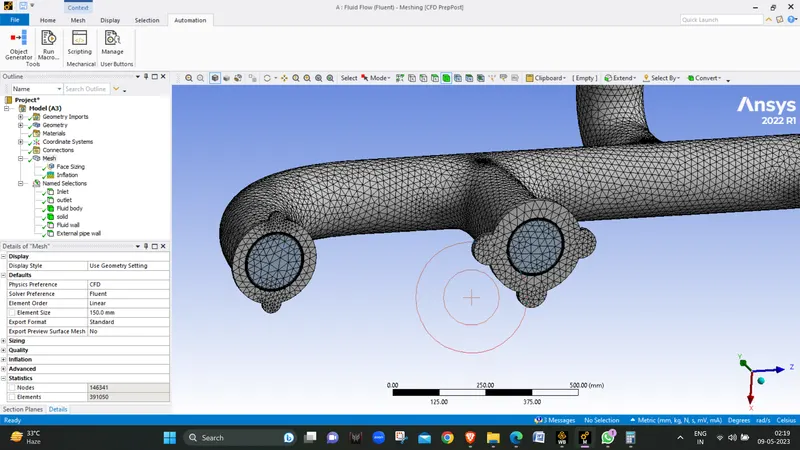
• now as we can se the transision of mesh elements is not good we will add a bodu sizing method to the fluid body with 20 mm element size.
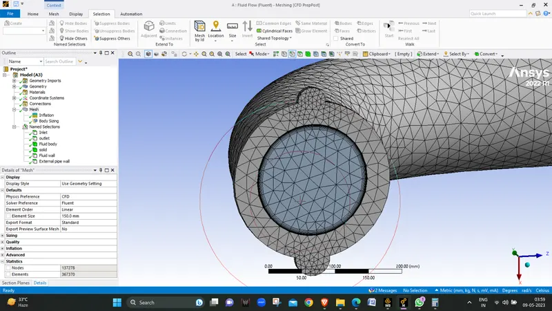
• We can see that the volume transition is still not good so we will now try to make the transition better by reseting the default mesh size to 250, increase number of inflation layer from 14 to 20 and give body sizzing as 15 mm element size. let see what the result comes out.
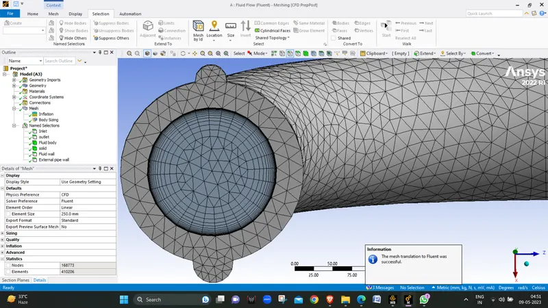
• We can see the volume transition is much better now, the total number of mesh elements created are 410206.
• Now we will go for the solver setup.

Solver Setup :-

• Open setup in the fluent module.
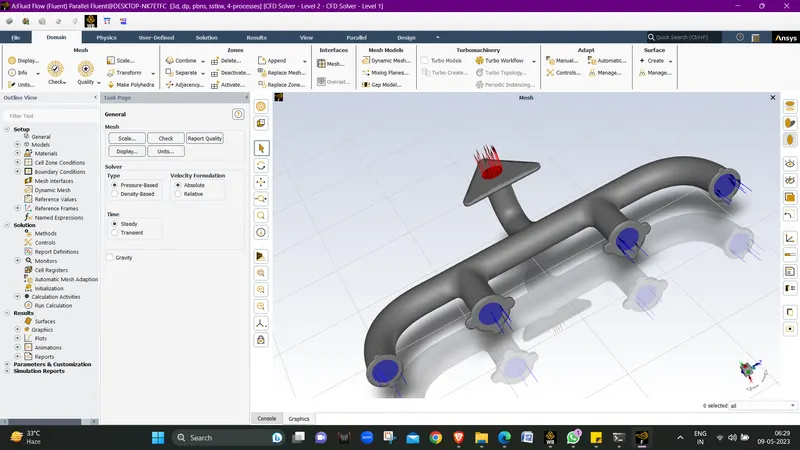
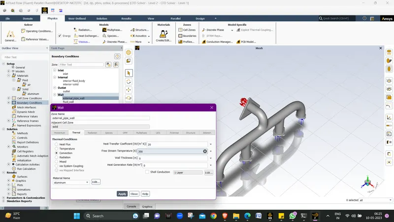
• We will be using K-omega SST model in this simulation and using working fluid as air with velocity of 5m/s considering the inlet condition of temperature as 700k and oulet as 300k and assign the external pipe wall with convection module setting up the heat transfer coefficient as 20 and the ambient temprature as 300k.
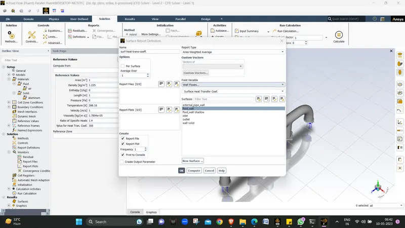
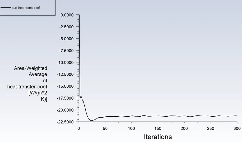
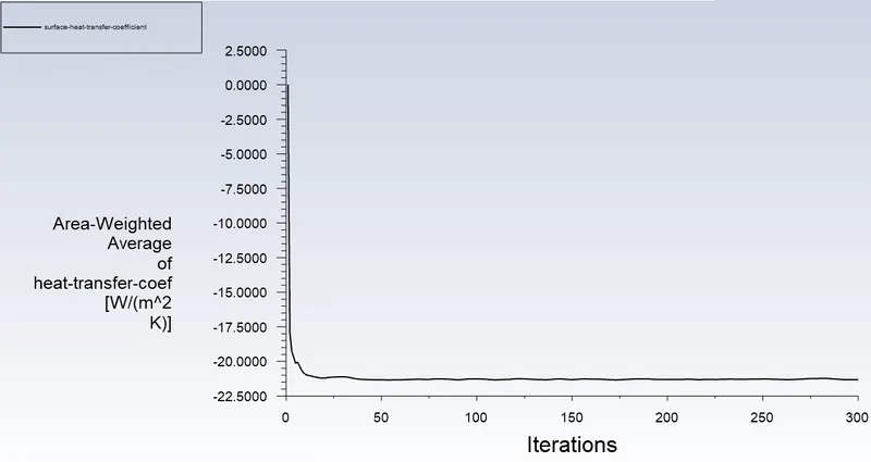
• we will now create definations for Surface heat transfer coefficient on the fluid wall under wall fluxes in Area waighted average and print to console.
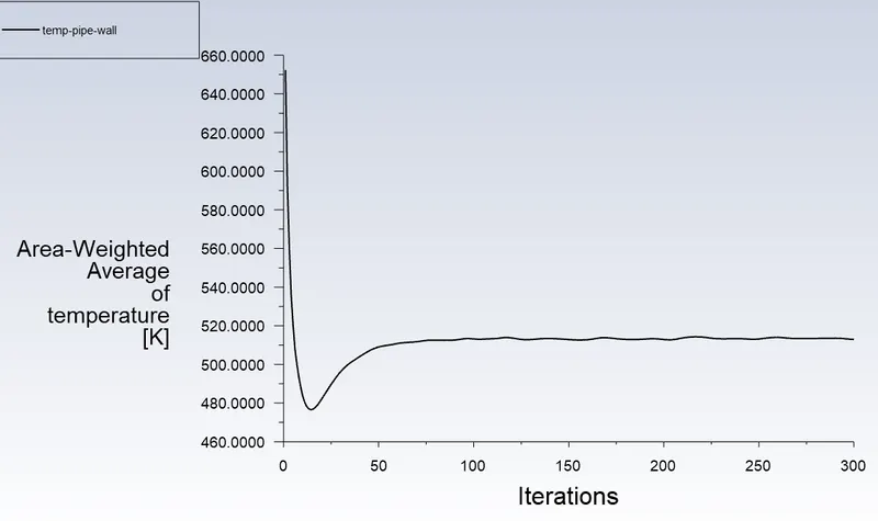
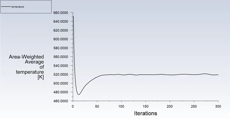
• Now we will add definations for Temperature at External pipe wall under Area weighted average.

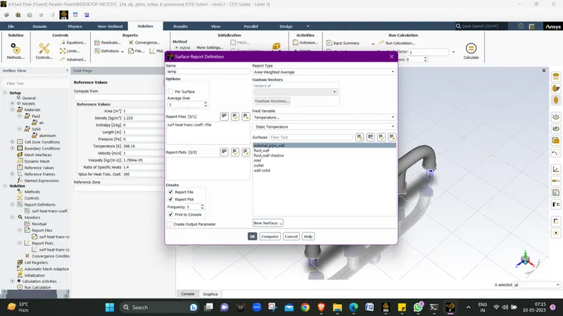
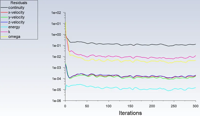
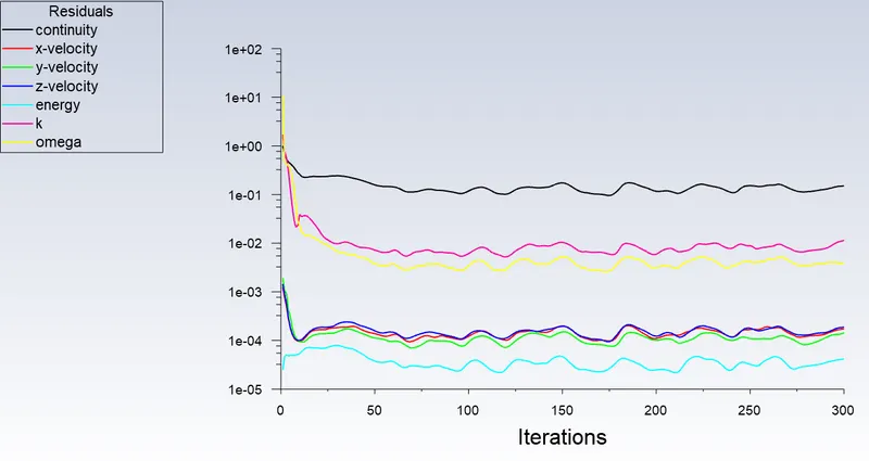
• Now we will initialize the simulation, once initiallization is done we will run claculation fro 300 iterations and check for sltion convergence. through graphs plotted due to simulation data.

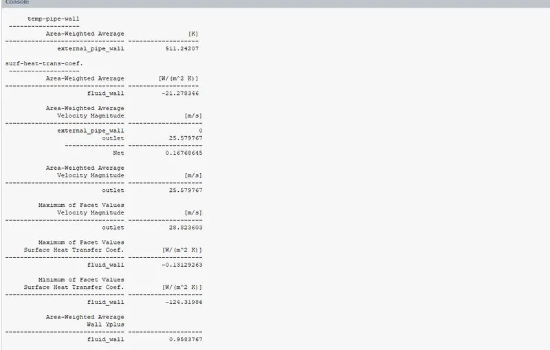
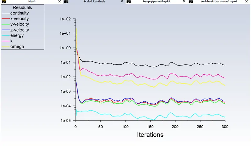
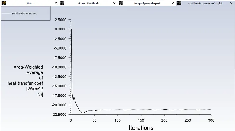
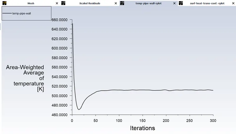
• We can see that the solution is now converged and we have computed some values through the simulation data.

• Area Weighted Average Temperature for external pipe wall :- 511.24207 K
• Surface Heat Transfer coefficient on fluid wall :- -21.278346 W/(m^2 K)
• Velocity Magnitude at outlet :- 25.579767 m/s
• Maximum of Facet Values for Velocity Magnitude at outlet :- 28.823603 m/s
• Maximum of Facet Values for Surface Heat Transfer Coef. on fluid wall :- -0.13129263 W/(m^2 K)
• Minimum of Facet Values for Surface Heat Transfer Coef. on fluid wall :- -124.31986 W/(m^2 K)
• Area-Weighted Average for Wall Yplus on fluid_wall :- 0.9583767
• we can now see that the values for surface heat transfer is in negitive magnitude because the heat is rejected from the fluid to the pipe wall therefore it is having negitive magnitude.
• Now we will go for contour plots and we will work on grid independent study by varying the mesh size.

Plots :-

Case 1:-

Default Mesh Size :- 250 mm

Body Sizing :- 15mm

Number of Inflation layers :- 20

Residual plot :-

Heat Transfer Coefficient Plot :-

Temprature at External Pipe Wall Plot :-

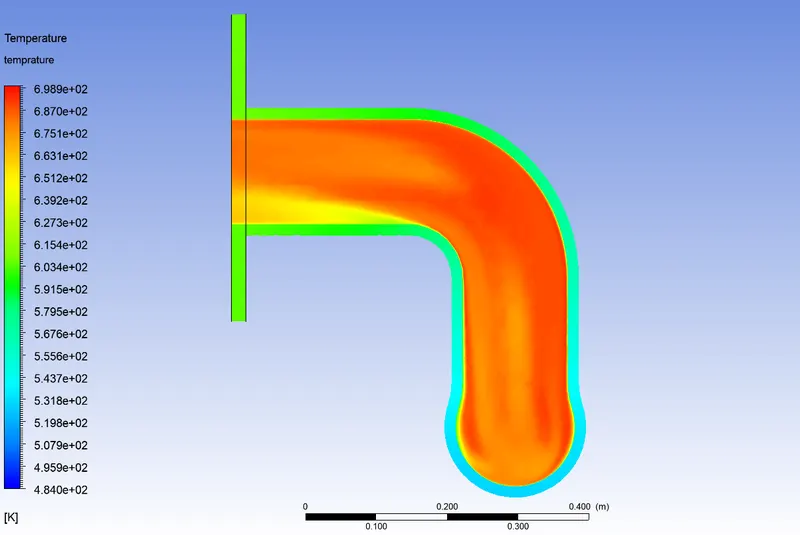
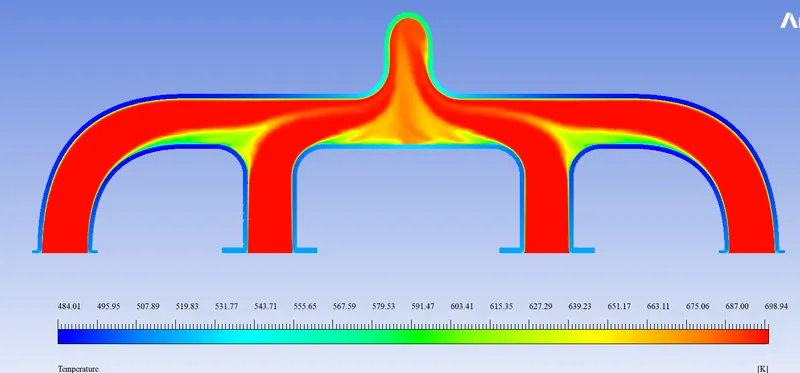
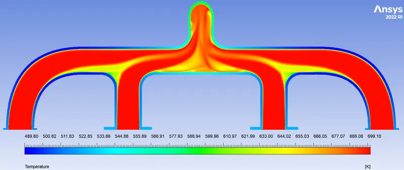
Temprature Contour Plots :-

view 1

View 2

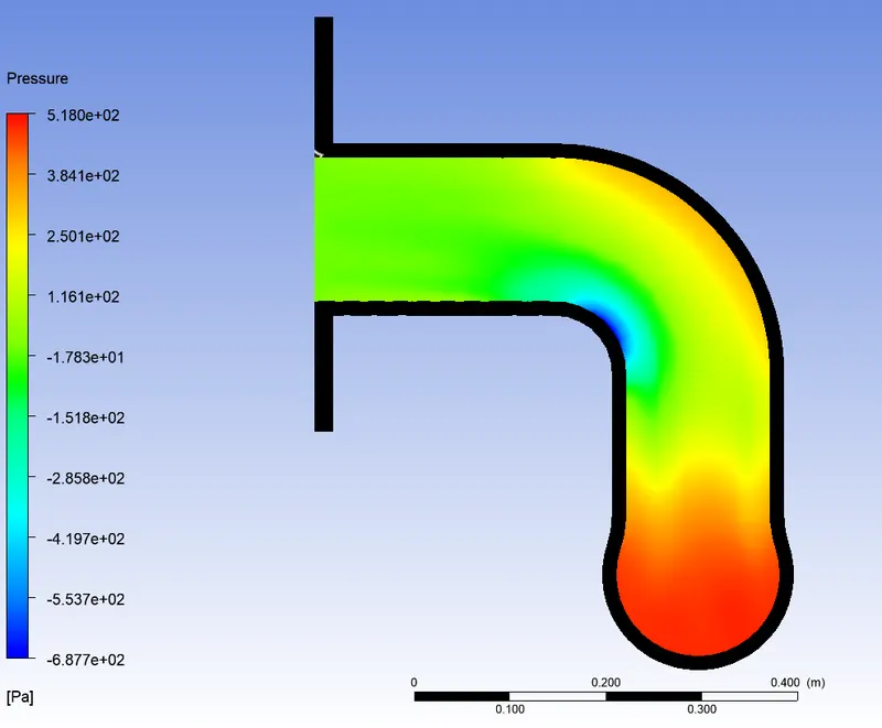
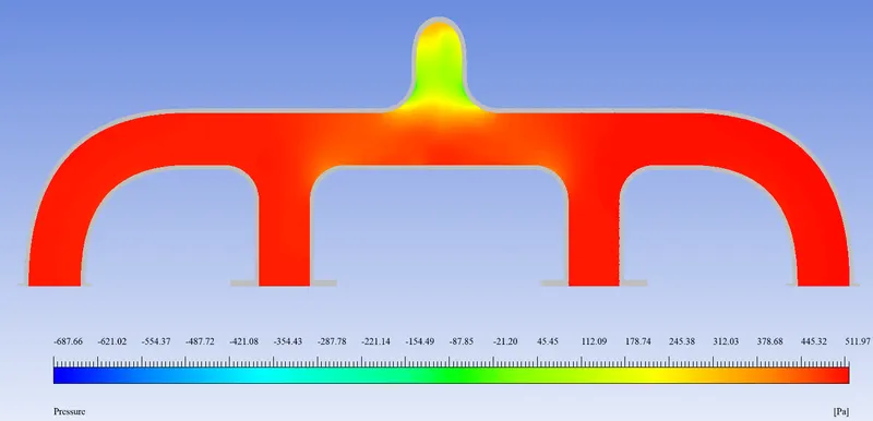
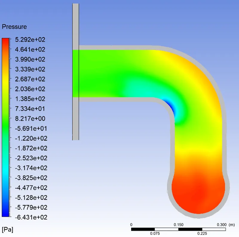
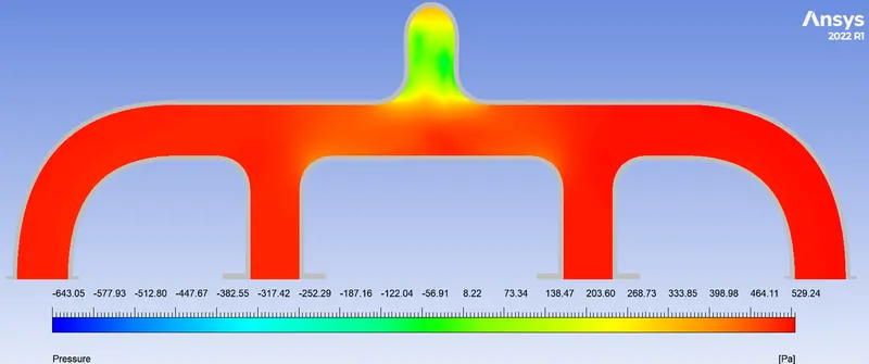
Pressure

View 1

View 2

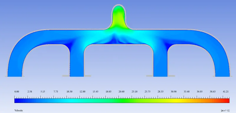
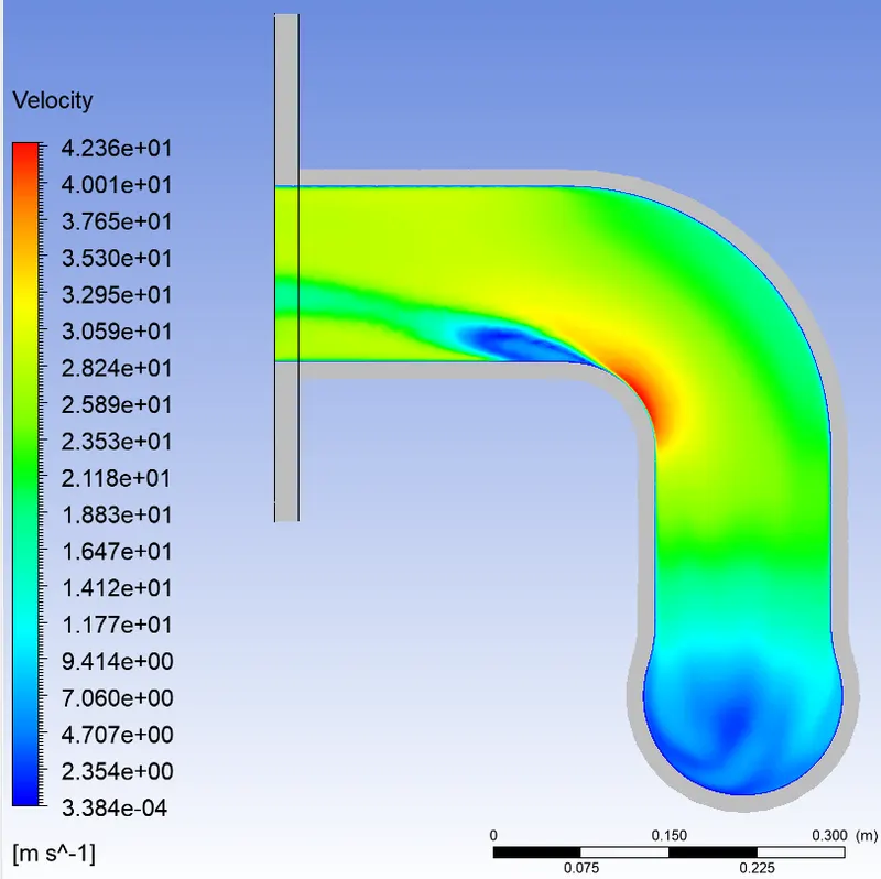
Velocity Contour Plots :-

View 1

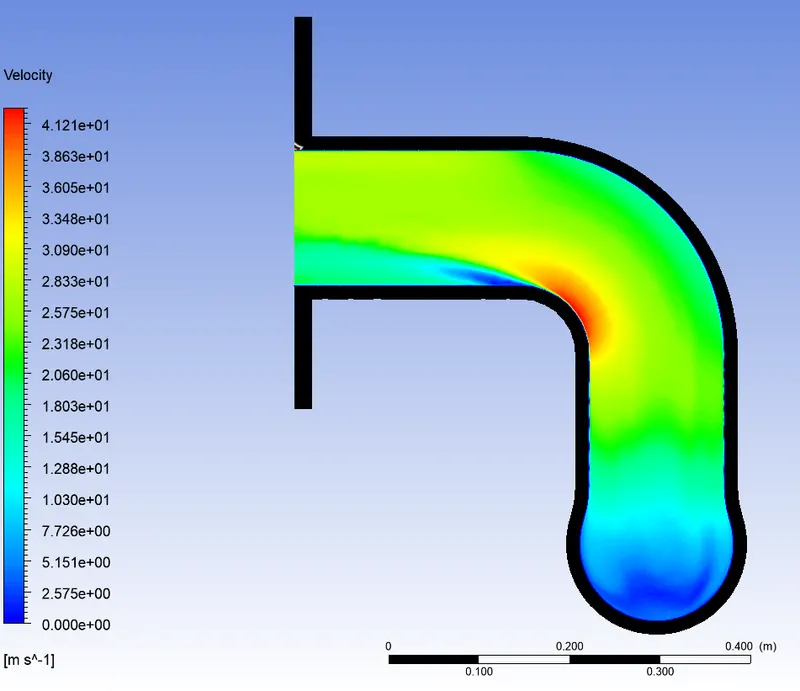
View 2

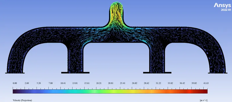
Velocity Vector

View 1

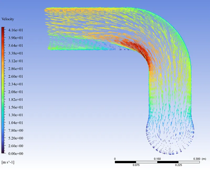
View 2

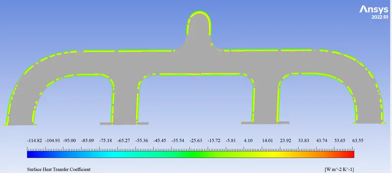
HTC Plot:-

View 1

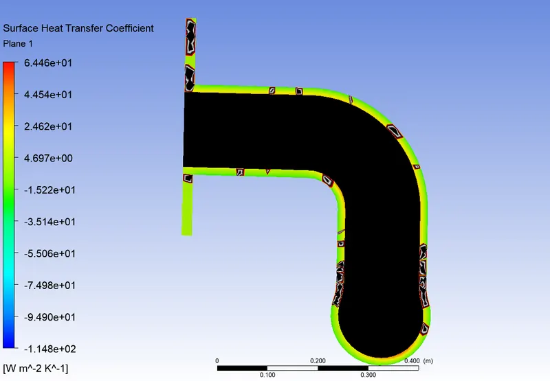
View 2

Case 2 :-

Default Mesh Size :- 225 mm

Body Sizing :- 10

Number of Inflation layers :- 18

Residual plot :-

Heat Transfer Coefficient Plot :-

Temprature at External Pipe Wall Plot :-

Temprature Contour Plots :-

View 1

View 2

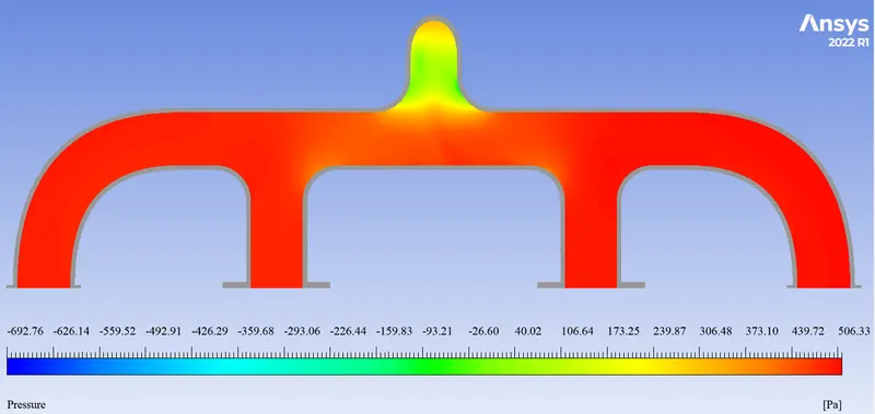
Pressure :-

View 1

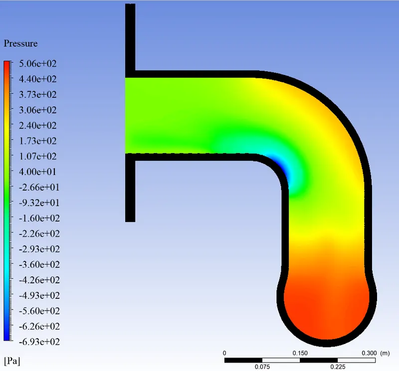
View 2

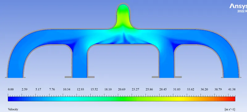
Velocity Contour Plots :-

View 1

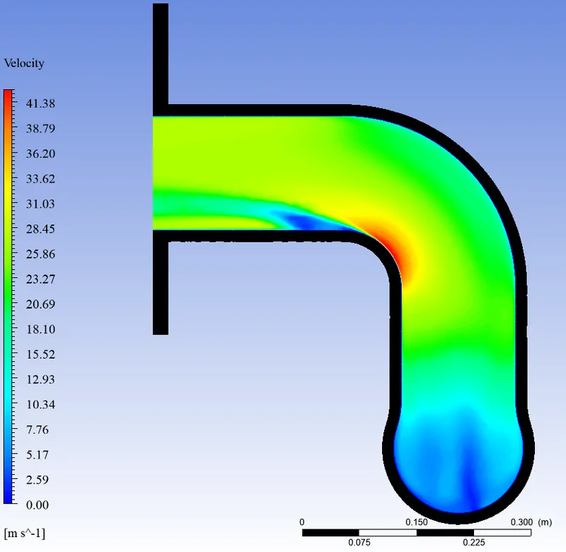
View 2

Velocity Vector

View 1

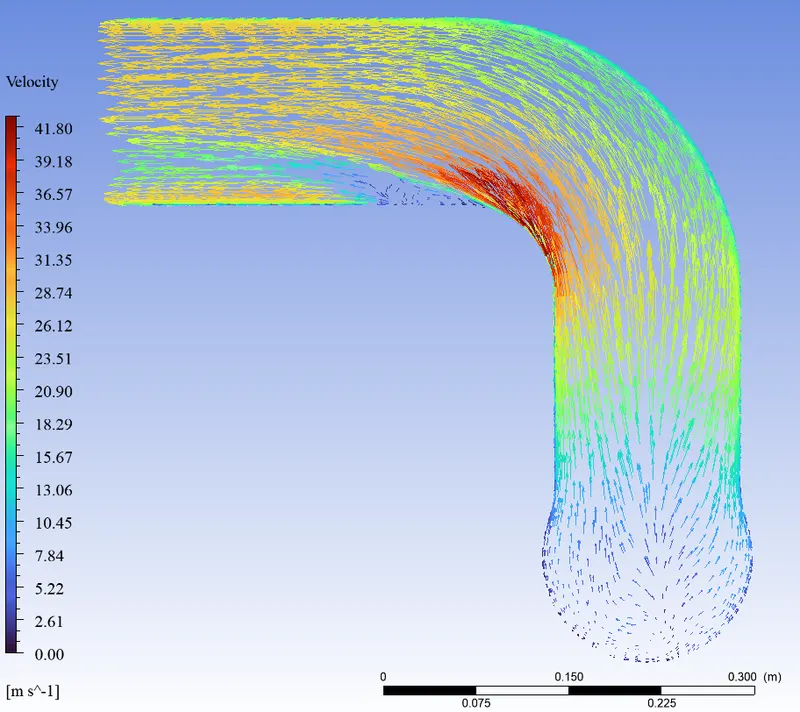
View 2

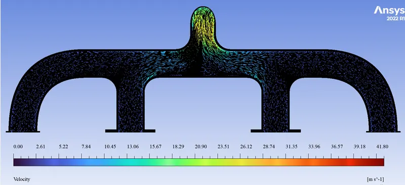
HTC Plot:-

View 1

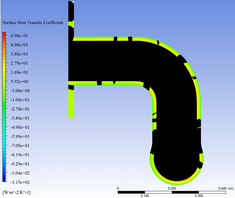
View 2

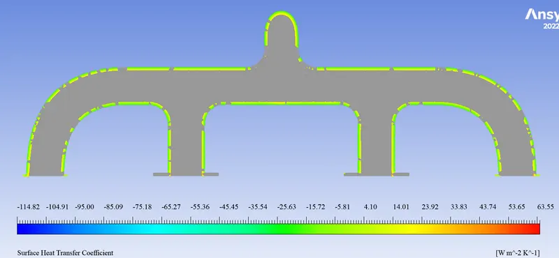
Case 3 :-

Default Mesh Size :- 200 mm

Body Sizing :- 7.5

Number of Inflation layers :- 18

Residual plot :-

Heat Transfer Coefficient Plot :-

Temprature at External Pipe Wall Plot :-

Temprature Contour Plots :-

View 1

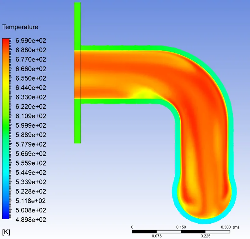
View 2

Pressure :-

View 1

View 2

Velocity Contour Plots :-

View 1

View 2

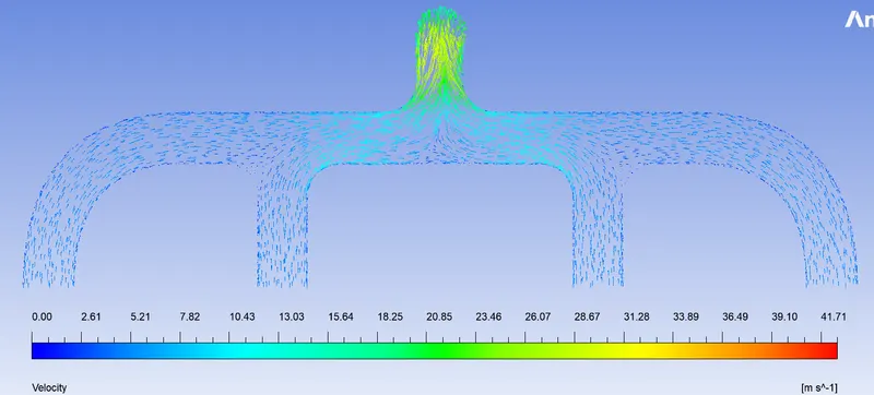
Velocity Vector

View 1

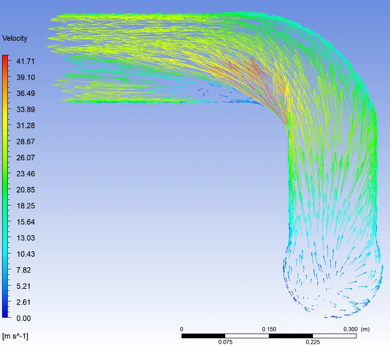
View 2

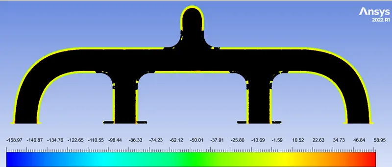
HTC Plot:-

View 1

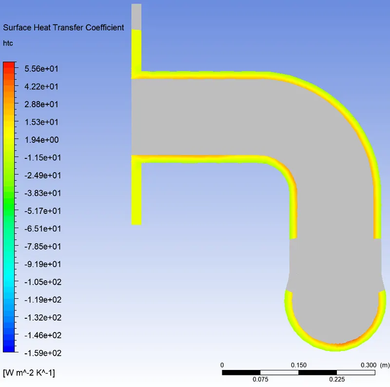
View 2

case 2

• Area Weighted Average Temperature for external pipe wall :- 511.24207 K
• Surface Heat Transfer coefficient on fluid wall :- -21.278346 W/(m^2 K)
• Velocity Magnitude at outlet :- 25.579767 m/s
• Maximum of Facet Values for Velocity Magnitude at outlet :- 28.823603 m/s
• Maximum of Facet Values for Surface Heat Transfer Coef. on fluid wall :- -0.13129263 W/(m^2 K)
• Minimum of Facet Values for Surface Heat Transfer Coef. on fluid wall :- -124.31986 W/(m^2 K)
• Area-Weighted Average for Wall Yplus on fluid_wall :- 0.9583767

Grid independent test :-

Cases	Mesh size (overall) mm	Body Sizing (mm)	No. of Prizum Layers	Cell count	Temp_Outlet (k)	Heat transfer coefficient W/(m^2 K)	Velocity magnitude (outlet) m/s
Case 1	250	15	20	410206	511.24207	-21.278346	25.579767
Case 2	225	10	18	1794370	512.94007	-21.264191	25.442013
Case 3	200	7.5	18	2916475	519.11023	-21.317151	25.829144

• There are notable changes in the three cases, mesh is more refined from case 1 to 3 to check the grid dependecy.
• A smoother mesh provides a more accurate results, from all 3 cases we can conclude that the flow is more defined at lower elemets size
• The finer the mesh gets, the easier it gets in visualizing the contours.
• we can see the velcity magnitude have increase with number of elements so we can take 25.829144 m/s as the final value for velocity magnitude.
• we can see that the temprture is increasing at oulet with increase in number of elements.
• we can see that the heat transfer coefficient is increasing slightly and the change can be considered as negligible.

Q How would you verify if the HTC predictions from the simulations are right? On what factors does the accuracy of the prediction depend on?

-> To verify the HTC preditions from the simulations are right or not we can perform several cases with different mesh size and different boundary condition, if the solution is converging at a point and refering studies related to the analysis we can predict whether the simulation is right and also using analytical methods.

The factors on which the prediction of simulation depends are :-

• Analyrical Methods
• Numerical Methods
• and experimental data