Week 4 - CHT Analysis on Exhaust port
AIM : To simulate CHT in ANSYS and study the results.
Introduction : The Conjugate Heat Transfer (CHT) analysis type allows for the simulation of heat transfer between solid and fluid domains by exchanging thermal energy at the interfaces between them.CFD Thermal Analysis extends the capability of FEA thermal analysis by replacing the simplistic convection boundary conditions with direct calculations of the heat transfer coefficients based on the fluid flow properties and is often referred to a conjugate heat transfer analysis.
CHT is used in various applications to study the effectiveness and various parameters associated with the heat transfer. it is used to analyze the exhaust port of automobiles, the effectiveness of air conditioning (HVAC), pumps and compressors, boilers, etc,.
Theory : Conjugate heat transfer corresponds with the combination of heat transfer in solids and heat transfer in fluids. In solids, conduction often dominates whereas in fluids, convection usually dominates. Efficiently combining heat transfer in fluids and solids is the key to designing effective coolers, heaters, or heat exchangers.
the main equations used in this model are
Q = -KA (dt/dr)
where,
Q = rate of heat transfer
A = area of contact
k = thermal conductivity
dt = temperature difference
dr = thickness of cylindrical wall
Nu =hD/K
where,
h = heat transfer coeficient
D = diameter of pipe
K = thermal conductivity
Nu =0.023*Re`wedge`0.8 * Pr`wedge`0.3
where,
Re = reynolds number
Pr = prandtls number
Procedure :
after startin workbench, the geometry is imported into the space claim and the geometry is prepeared for meshing.
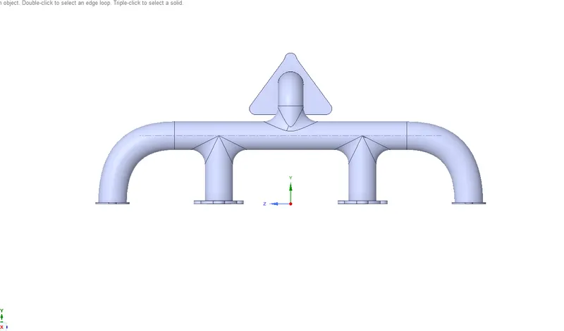
The unwanted extra edges of the geomtry is removed using the extra edge tool in the repair option.
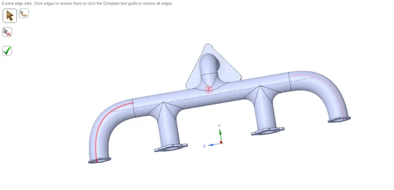
after clearing the unwanted edges the internal volume is extracted using the volume extract option.
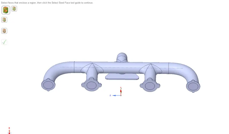
after extracting the volume enable share tolopology in workebench. then proceed to the meshing.
in ANSYS mesh name the inlet, outlet, fluid domain, fluid wall and pipe wall.
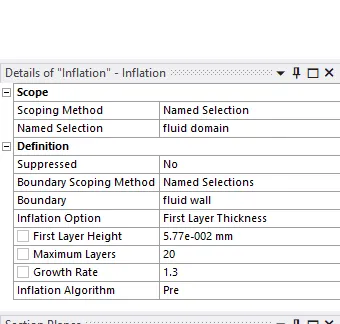
after naming mes the geometry and create inflation in the fluid domain inorder ot analyze the heat transfer coefficient.
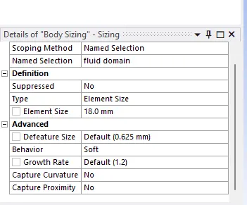
the inflation layer is created with accordance with the y+ value. and the first layer thickenss is calculated from the Y+ calculator. the minimum number of inflation layer is found out from the Y+ calculator. the number of inflation layer is incfeased in order to match the size of the mesh in the fluid domain. also body sizing is used to control the fluid domai mesh size.
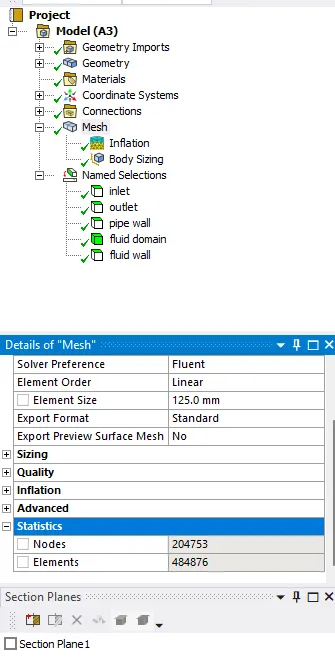
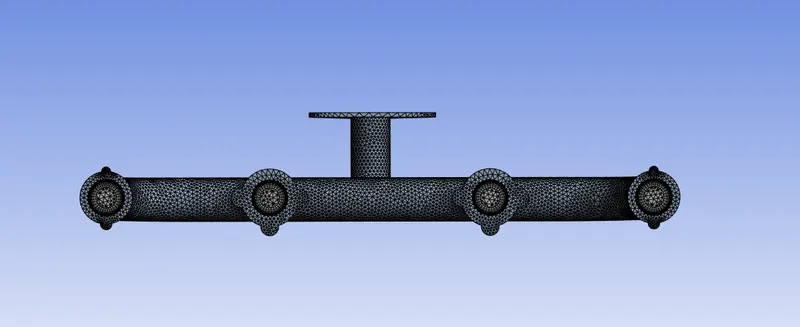
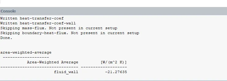
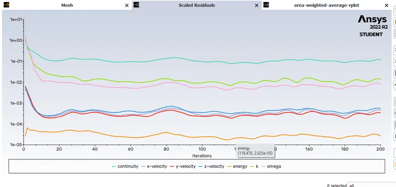
after creating the mesh and inflation layer in fluent define the inlet parameters and outlet parameters. enable energy equation. and then create report for the area weighted average for heat transfer coeficient at the fluid wall. run the simulation in steady state using - omega SSt solver. then run the iteration for 200 iterations and chec for convergence.
case 1 : Y+ = 1
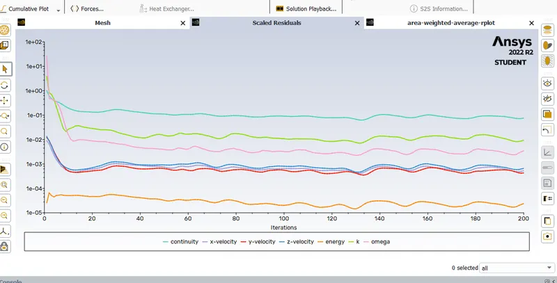
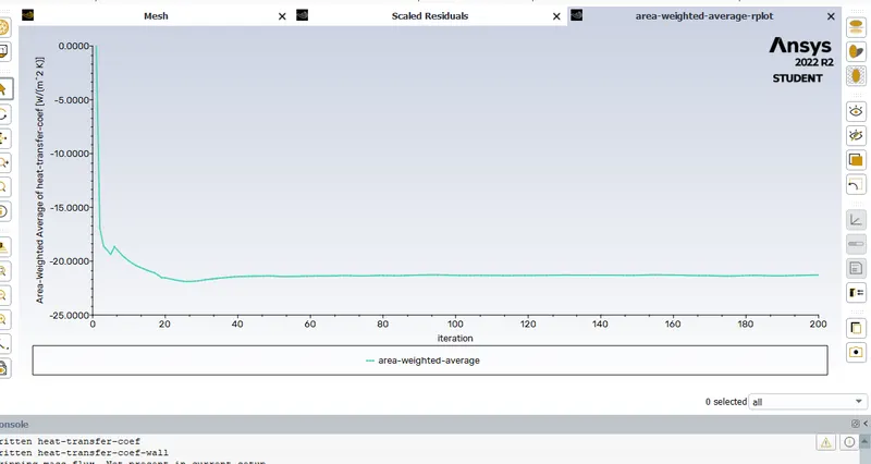
after the solving go to solution to plot the velocity and temperature contours in the results.
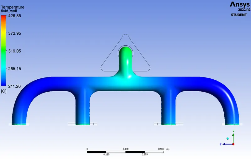
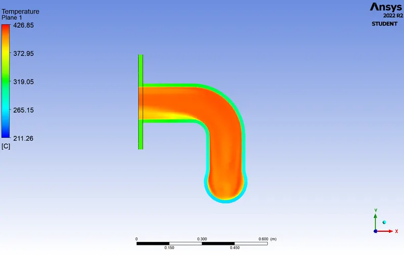
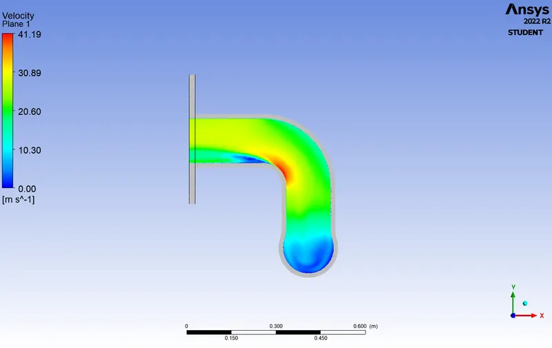
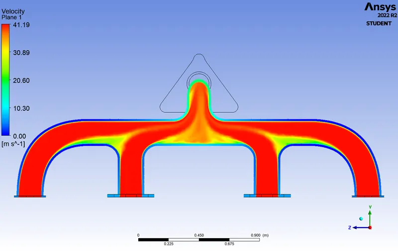
case 2 : Y+ = 3
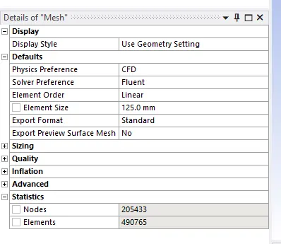
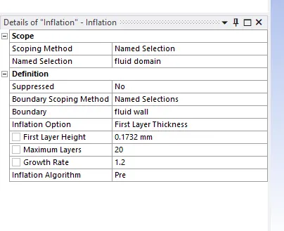
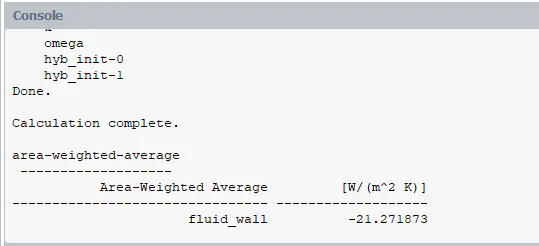
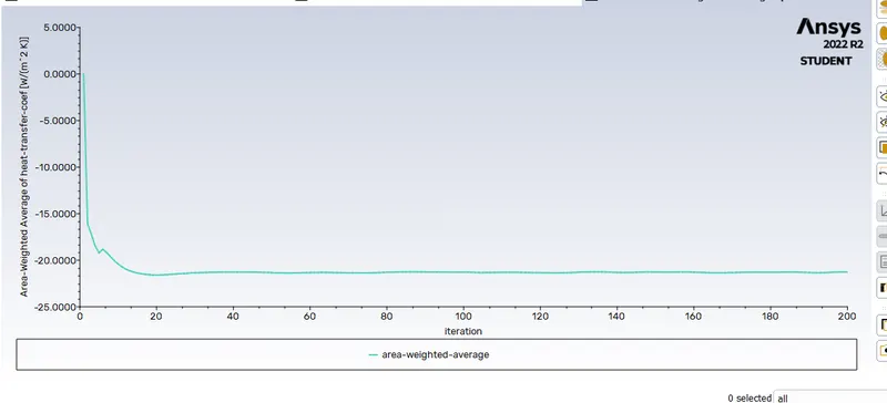
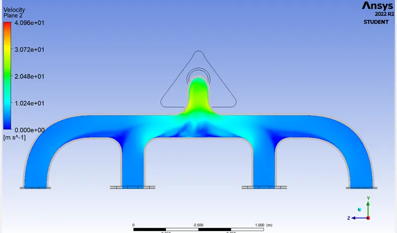
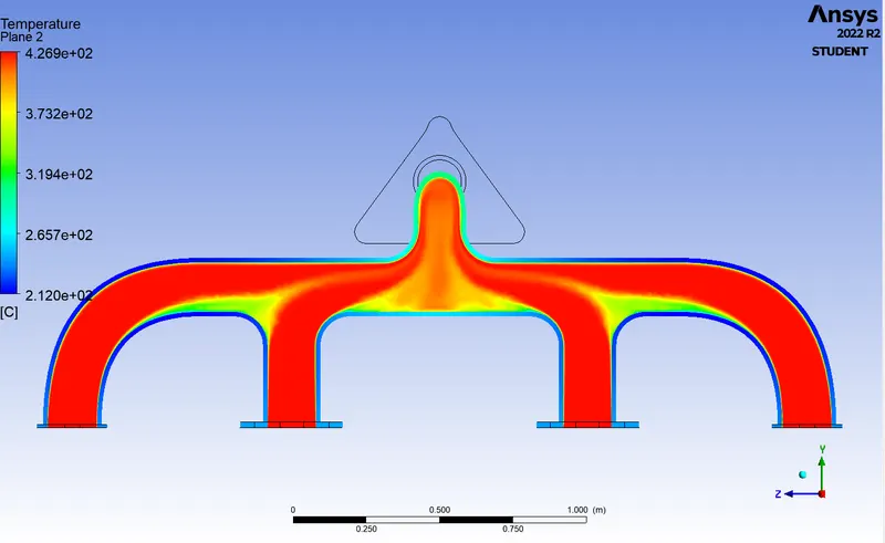
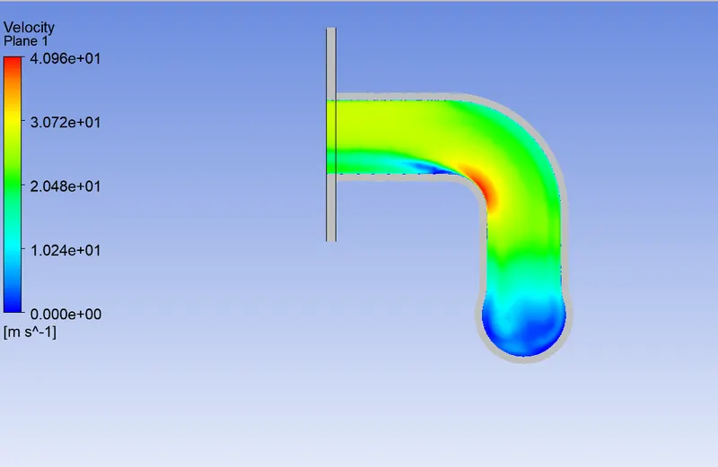
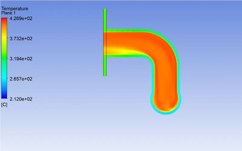
Result : the CHT analysis was done and the results obtained was compared with the results from the numerical caluculation. the heat transfer coefficient calculated numerically was 19.16.
| case | Y+ value | Cell count | mesh size | no. inflation layer | h value |
| 1 | 1 | 484876 | 125 mm | 20 | -21.2763 |
| 2 | 3 | 490765 | 125 mm | 20 | -21.2718 |
Conclusion : the CHT simulation suing ANSYS wwas studied adn the results was compared. There is variationn in the heat transfer coefficient computed from the simulation and that computed from numerical calculation. this variation is due to the non inclusion of change in diameter of the various inlets and outlets. also the coeft of heat transfer varies along the pipe. the error obtained is within the limit.