Week 4 - CHT Analysis on Exhaust port

AIM: To analyze Conjugate Heat transfer through an Exhaust Manifold.

OBJECTIVES:

• Discuss the importance of Conjugate Heat Transfer.
• Simulate the Exhaust port model in fluent while maintaining the proper Y+ value according to the turbulence model.
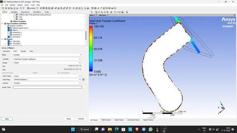
• Calculate the wall/surface heat transfer coefficient on the internal solid surface & show the velocity & temperature contours in appropriate areas.
• To verify the HTC predictions

INTRODUCTION:

Conjugate heat transfer is defined as the heat transfer between two domains by the exchange of thermal energy. For a system the thermal energy available is defined by its temperature and the movement of thermal energy is defined by its heat flux through the outer walls. Heat transfer in solids happens through conduction, through the walls by convection, and in the liquid phase through convection.

CHT provides the temperature prediction and the hotspot regions at the solid-liquid interface and we can also accurately predict the heat transfer, for example, conduction through solids, convection through fluid, and thermal radiation. It also provides the velocity and pressure distribution of the fluids moving inside in the solid. We can also use CHT in design optimization for the improvement of heat transfer and cooling capacity.

CHT can be used in turbochargers, engine equipments, HVAC, exhaust ports and heat ejection through electronic devices, etc.

Heat transfer coefficient (h):

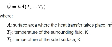
The heat transfer coefficient, in Thermodynamics, is the proportionality constant between the heat flux and the thermodynamic driving force for the flow of heat

the heat transfer rate is:

SETUP:

GEOMETRY:

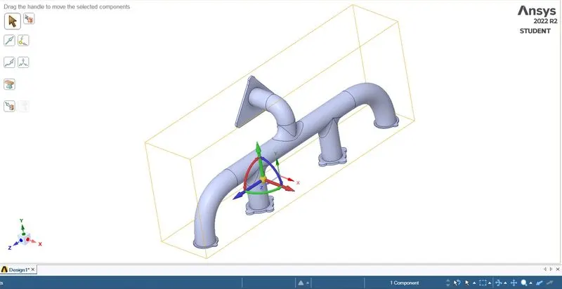
• Load the CAD model of the Exhaust manifold in Spaceclaim and check for any extra edges, remove them if any.
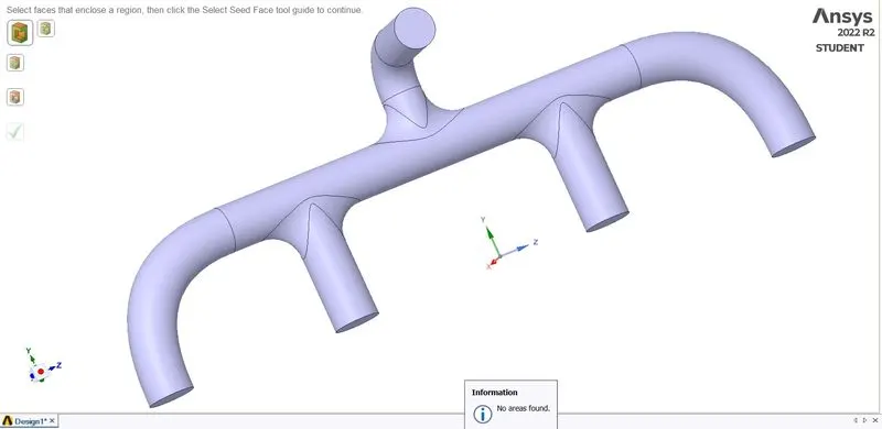
• Go to Repair > Volume extract, and select the edges to separate inner and outer volume. Name the outer volume as Solid volume and the inner ass Fluid volume and move both the volume to a new component and delete empty components the fluid volume for the port will be generated and can be seen below.
• Go to workbench > Shareprep, to share the physics between the fluid and solid volume, and conformal mesh can be achieved. pink circles are seen after completing the process.

MESH:

Open the mesh tab and select the geometry and named the parts:

• Inlet
• Outlet
• Outer Wall Convection

Ansys fluent automatically adds an unnamed part as a wall and an adiabatic boundary condition is applied. Select the mesh and generate a base mesh of a default size of 150 mm.

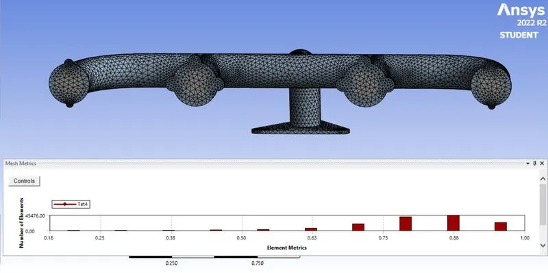
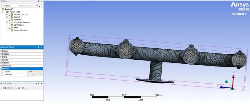
Here the default element size for this mesh is 150mm and the total number of elements is 137770 and the number of nodes is 27466. Further, the mesh quality was also good with the maximum number of elements at 88% quality. The mesh quality can be seen below:

Setting Up the Physics

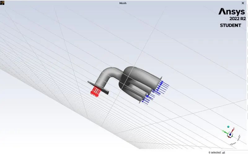
Once the mesh has been created without any errors we will proceed with setting up the physics. First, we will start by checking the mesh and then we will start with defining the solver. We will define the solver as the k-epsilon mode along with the energy equation. After that, we will define the materials as the solid exhaust port as aluminum and the fluid as air. Further, the boundaries conditions will be defined as shown below:

CASE 1: BASE MESH

The setup involves the following changes to the solver.

1. Solver - pressure-based solver
2. solver state - steady state
3. Turbulence Model - K-epsilon with standard wall function
4. boundary conditions

• Inlet velocity = 5 m/s
• Heat transfer coefficient = 20 W/m^2K
• pressure outlet = 0 pascals

RESULTS:

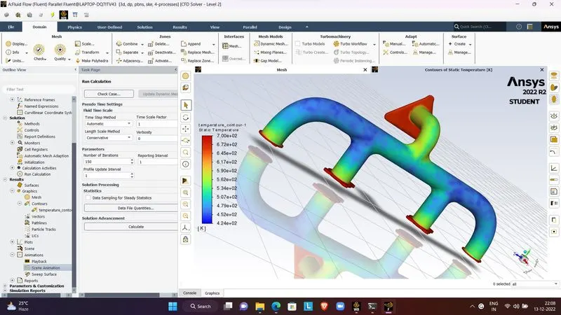
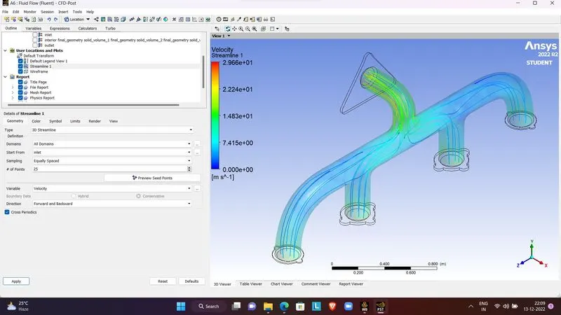
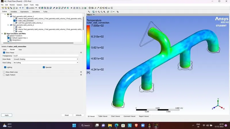
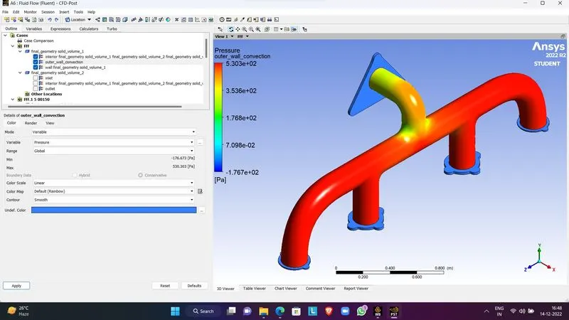
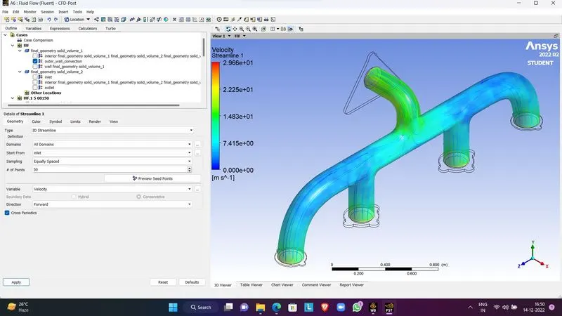
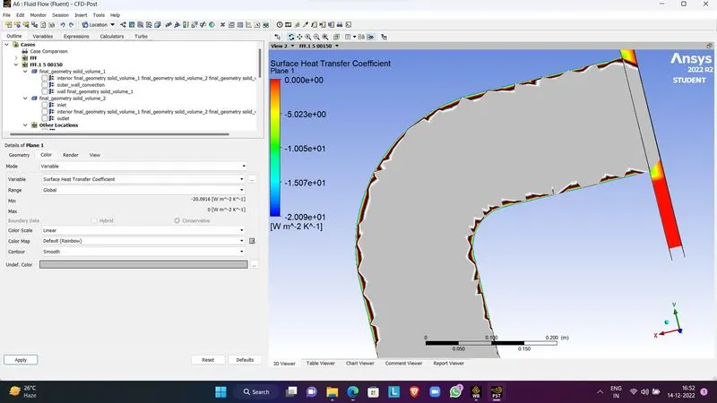
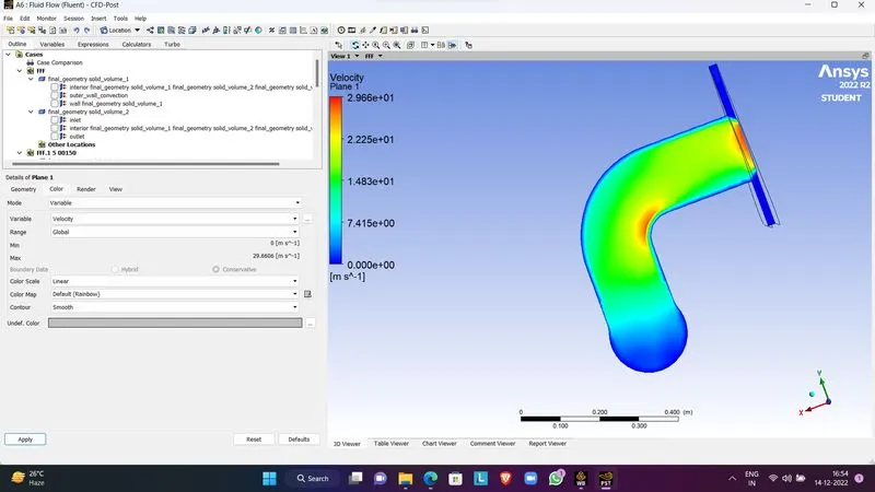
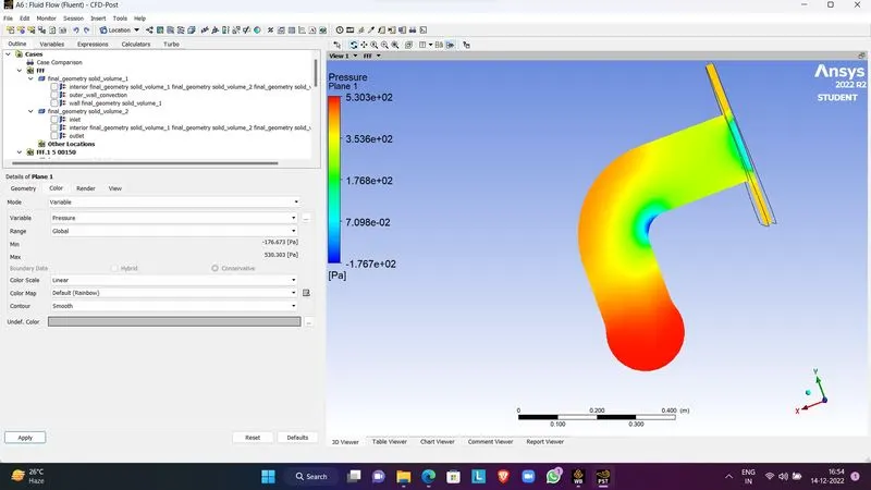
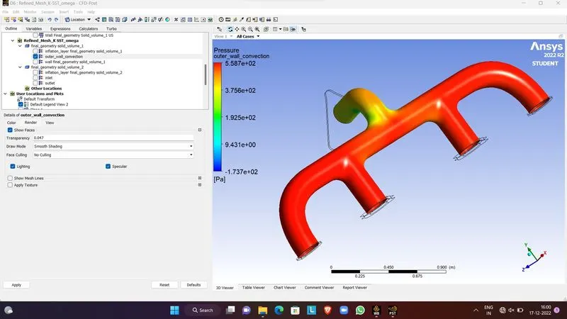
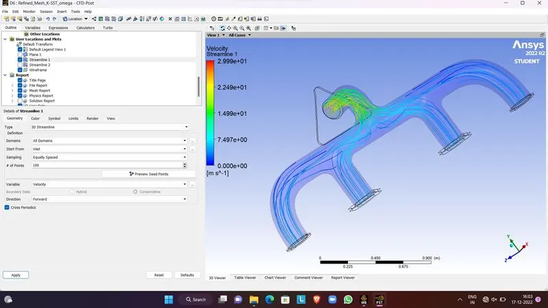
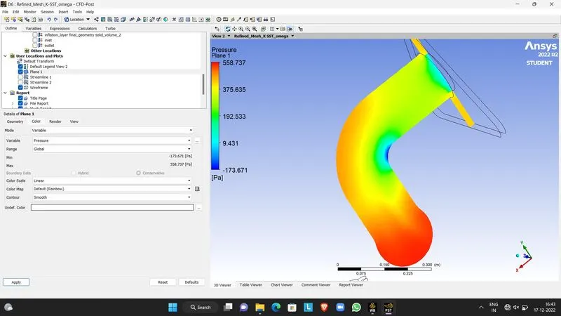
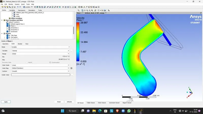
During the velocity distribution at the midplane, we can notice that the velocity at the bend is maximum near the turning, and apart from that the pressure decreases and the velocity increases as the fluid moves towards the outlet. Also, the maximum pressure can be seen at the bend as seen in the contour.

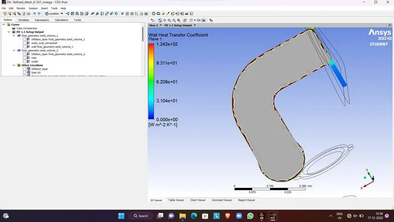
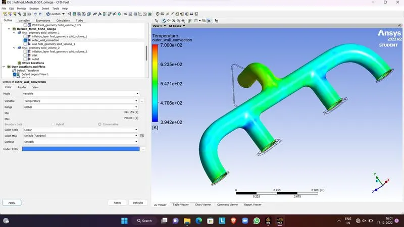
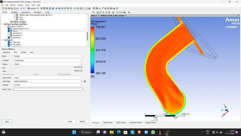
In an exhaust port analysis the hot air enters from the inlet and then it transfers its heat from the convection to the exhaust port body and then it transfers it heat through conduction all along the body of the port. Here in the baseline mesh, the results are seen as expected because the temperature of the exhaust port should rise when all the inlets combine with each other near the outlet pipe. In the heat transfer along the convection plot, it can be seen irregular near the walls due to the coarser mesh along the walls and also the heat transfer coefficient along the walls also the heat flux is about 25 in the plot shown in the area average. This can be due to the coarser mesh and the turbulence model being used is k epsilon which is generally used in between the Y+ of 30 to 300. Further, we will now proceed with the refined mesh and reduce the mesh size near the walls to maintain the accurate y+.

CASE 2: REFINED MESH

As the baseline mesh doesn't have an inflation layer catching the wall heat transfer coefficient will not be accurate. So in order to catch the phenomena near the wall condition the best choice is to construct an inflation layer and Use the k-omega SST turbulence model. Combination of these along with proper y plus value we can get near to the experimental value.

Now hide the outer body and select the inner face and named it as the inflation layer. Go to the inflation layer and select the inflation layer and maximum thickness of 5 mm.

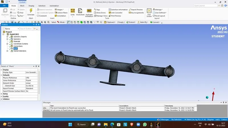
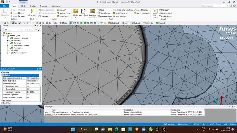
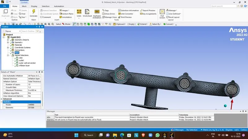
The setup involves the following changes to the solver.

1. Solver - pressure-based solver
2. solver state - steady state
3. Turbulence Model - K-SST Omega.
4. boundary conditions

• Inlet velocity = 5 m/s
• Heat transfer coefficient = 20 W/m^2K
• pressure outlet = 0 pascals

RESULTS:

'

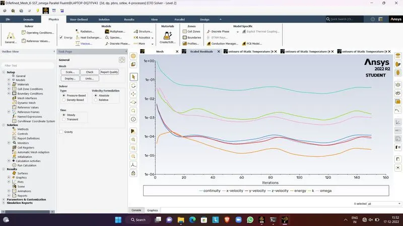
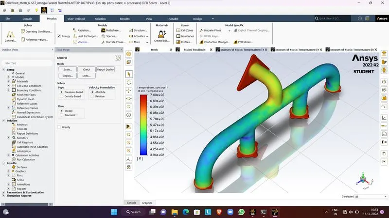
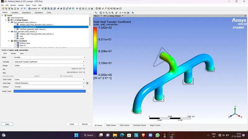
Verify HTC :

Under forced convection circumstances, we can determine the heat transfer coefficient by using the Dittus-Boelter correlation. Using the Dittus-Boelter correlation the heat transfer coefficient can be calculated in the following way using two further dimensionless groups, the Reynolds number, and the Prandtl number:

h = (k/D_H)*Nu

where k is the thermal conductivity of the liquid, D_H is the Hydraulic diameter, and Nu is the Nusselt Number which is determined by the following equation:

Nu = 0.023Re^0.8Prⁿ

where, n= 0.4 when fluid is being heated

n= 0.3 when fluid is being cooled

In this equation, Re is the Reynolds number which equates to:

Re = (m D_H)/(μ)

Pr is the Prandtl number :

Pr = (C_p* μ)/k

For the Reynolds number, m is equal to the mass flow rate. For the Prandtl number, C_p is equal to heat capacity, and in both equations, μ is the viscosity of the fluid in consideration. Once we have all of these factors, we can get a decent estimation of the heat transfer.

Factors affect the quality of prediction:

• More refined mesh leads to better results.
• Use inflation layers and apply proper Boundary conditions.
• Proper selection of turbulence model according to y+ values.

Conclusion

1. The results are more accurate in the second case as compared with the first case due to the mesh refinement.
2. There is no change in temperature difference in both cases but the change in minimum temperature, is in the second case because of mesh refinement.
3. The wall coefficient heat transfer also increases in the second case.
4. The velocity and hence the Reynolds number, is higher at the outlet. Due to that, the heat transfer and temperature is higher.
5. The heat transfer coefficient is higher between fluid and solid at the outlet pipe, because the velocity of the fluid is higher