Week 4 - CHT Analysis on Exhaust port
AIM :-CHT Analysis on Exhaust port
Objective :-
In this challenge,
1. brief description of why and where a CHT analysis is used.
2. simulate both fluid flow and also the heat transfer to the solid i.e., CHT Analysis on an Exhaust port
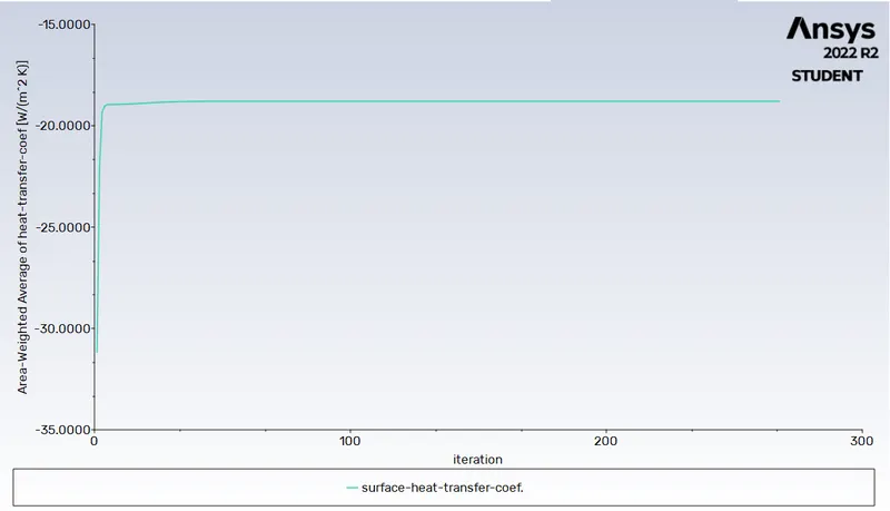
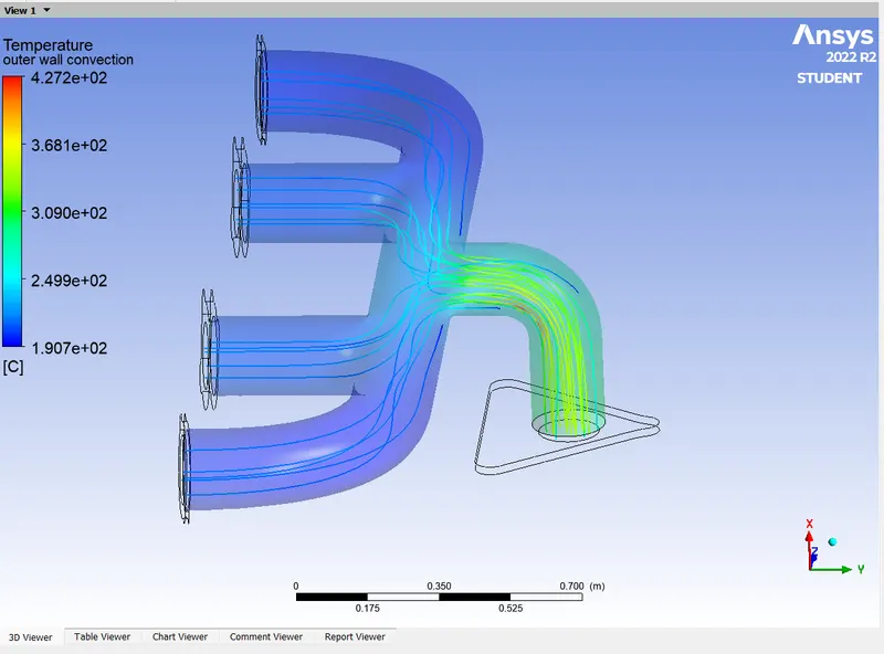
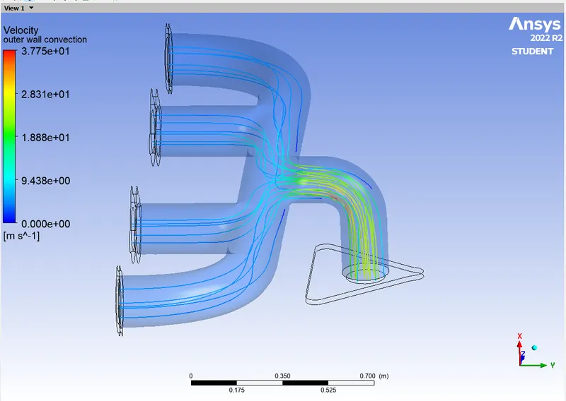
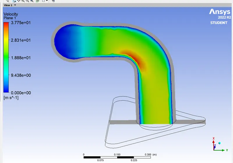
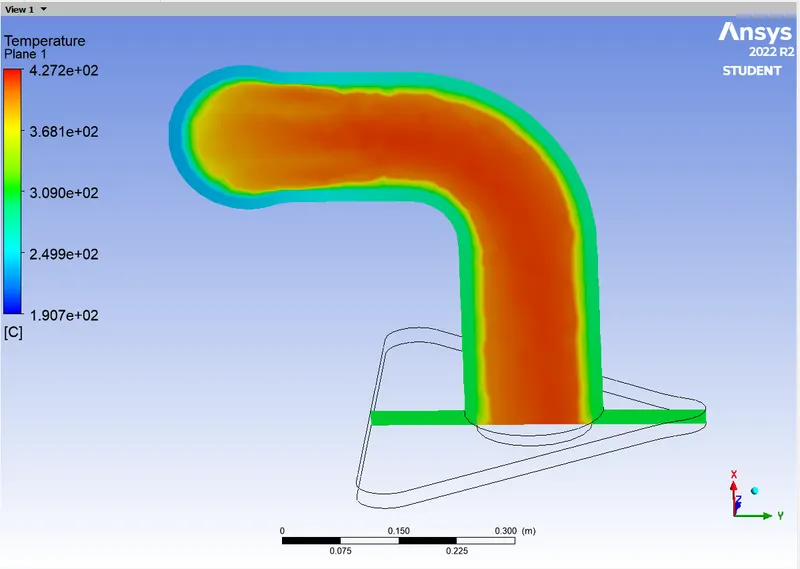
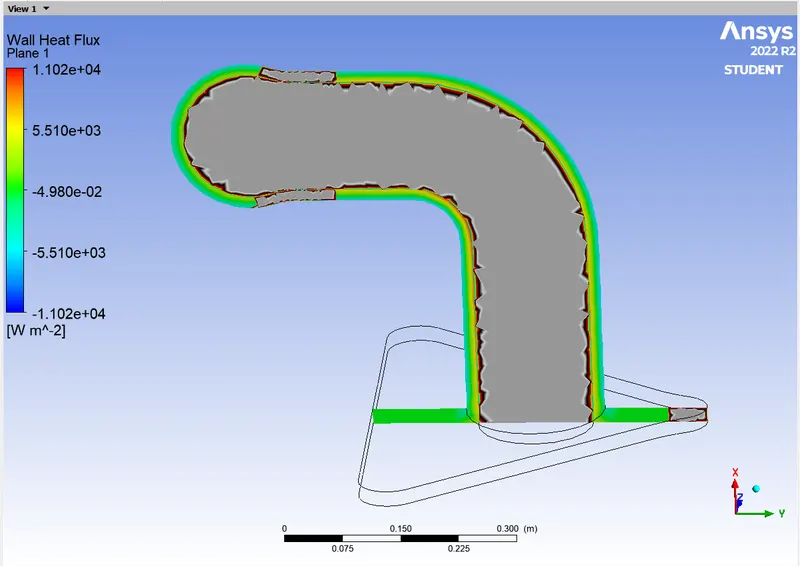
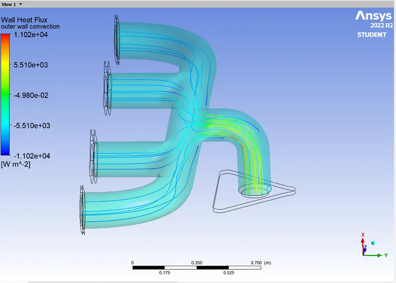
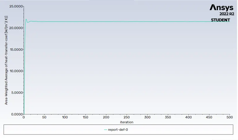
3.calculate the wall heat transfer coefficient on the internal solid surface & show the velocity & temperature contours in appropriate areas.
4. verify the HTC predictions from the simulations are right? And mention the factors that the accuracy of the prediction depend on.
Conjugate Heat Transfer (CHT) analysis :-
Conjugate Heat Transfer analysis allows for the simulation of heat transfer between solid and fluid domains by exchanging thermal energy at the interfaces between them and transported via conduction within solids and adiditionally via convection within fluid domains.
Geometry setup :-
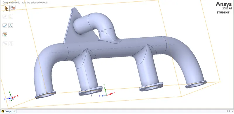
In fluent module we have to open spaceClaim and import the geometry.if you look closely to the geometry it has solid part .So first let us extract the fluid volume.
For that we have to go to,
prepare -> volume extract -> select edge selection -> then select all the edges of inlet and outlet -> then click ok.fluid volume will be created .
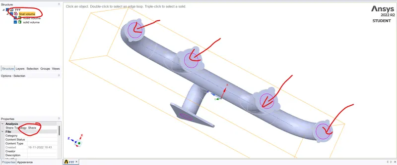
we need to share topology.
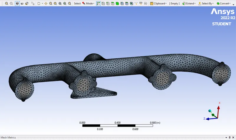
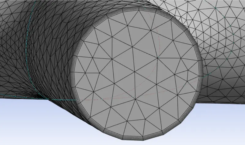
Now if you open meshing and you will see that there is perfect mesh connectivity and the interface is shared perfectly.This is exactly how we need to make meshes for CHT simulation.
This completes the creation of geometry.Then we close the spaceClaim ,the progress will be saved automatically.
Meshing :-
For meshing we open Meshing,where we mesh our model so that we can use it to solve our model.
In general it is always good to name the surfaces before meshing. So let us do that. We first select the entity by using the entity selection by using faces so that we can provide name for our entity selection.
steps : select the edge you want to name by using edge selection -> then press N -> name the selection.
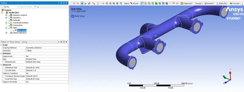
Sizing(Body sizing) :-
Problem Setup :-
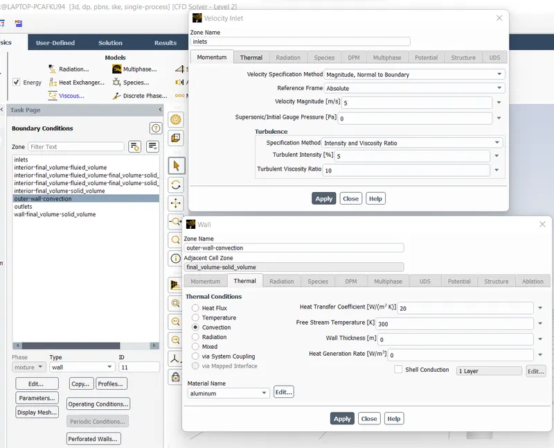
To set up our problem we open Fluent and setup inital conditions , boundary conditions material etc.,
We first start with checking the mesh quality using perform mesh check under domain.If no error is seen in console window then we can proceed further.
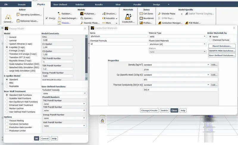
Then we move move to setting up physics where we select the solver ,viscous model ,initial and boundary conditions etc.,
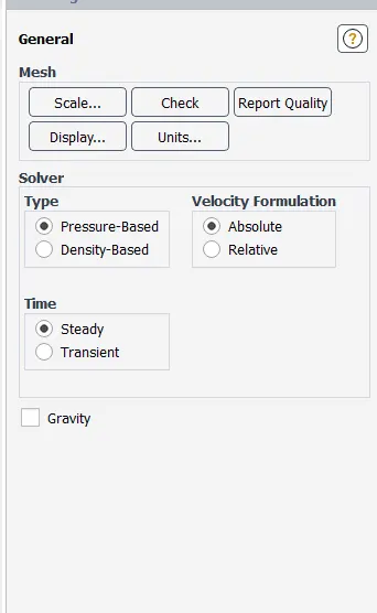
We use a steady state pressure based solver to solve our model.
Physics :-
Boundary Condition :-
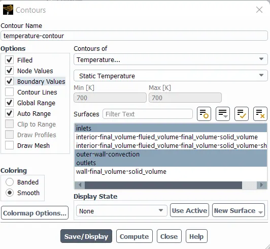
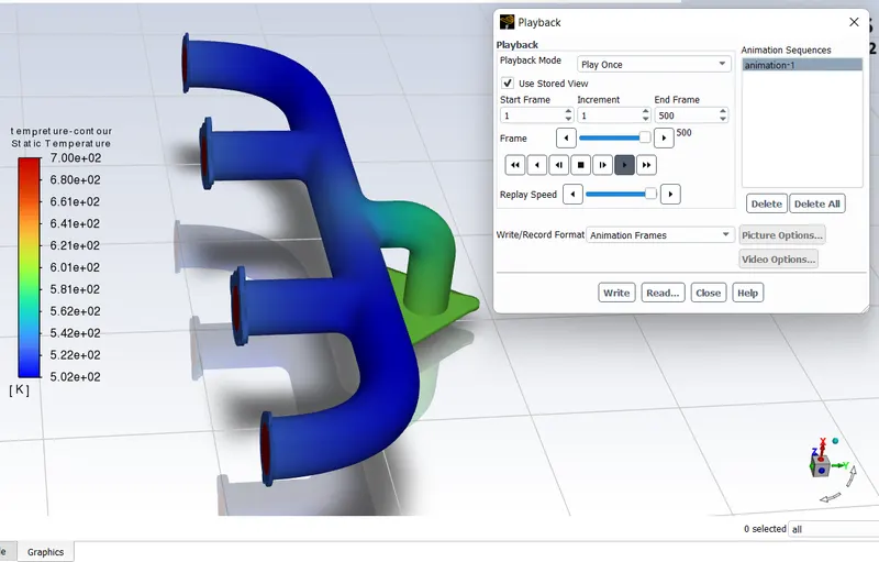
Now we want to see the temperature contour.
For contour -> go to solutions tab -> graphics -> contour -> in contour of : select temperature under that select static temperature -> select the outer walls and press save /display.
Solving :-
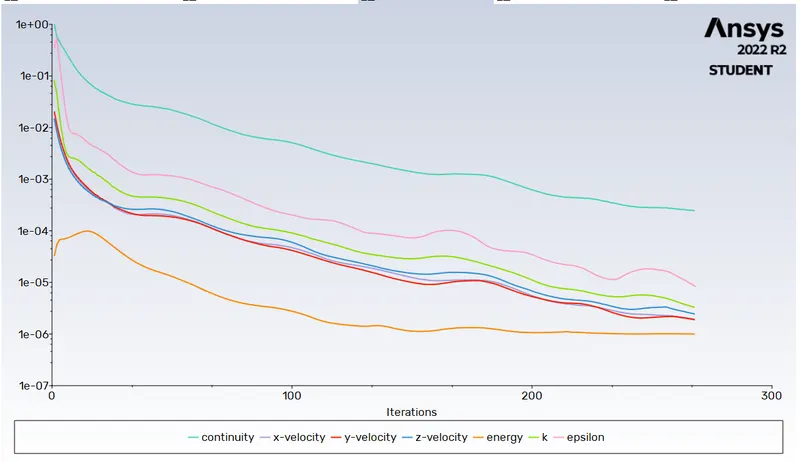
Give iterations such that your solution is converged.
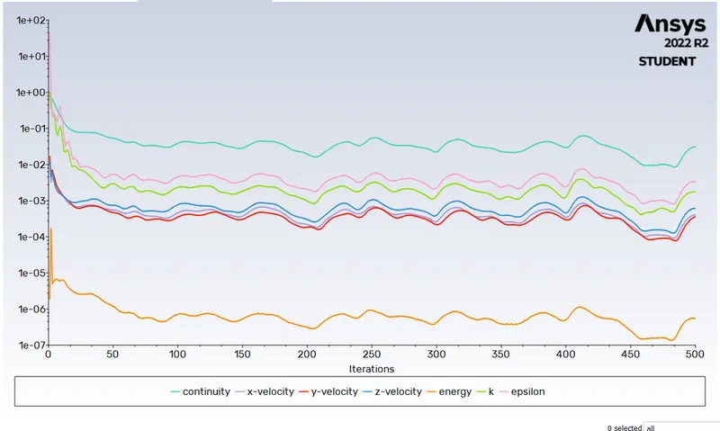
Run the simulation until the steady state is reached.Lets run for 500 iterations ,we can find the solution is converged.
Then we can see that in the residual plot that residuals dropping and reach a steady state after 100 iterations.
Then let us post process the results.
Post processing :-
Residuals plot
Refind mesh :-
https://drive.google.com/file/d/1BQBkJczSmN3ONgKW3pIACHlk88bgzabq/view?usp=share_link