Week 4 - CHT Analysis on Exhaust port
AIM: To analysis conjugate heat tranfer through an exhaust manifold to calculate the wall and surface heat transfer coefficient on the internal solid surface.
INTRODUCTION:
In the computational fluid dynamics and more specifically conjugate heat transfer (CHT) analysis can accurately predict heat transfer by simultaneous solving all the relevant solid and flow field heat transfer processes, for example: conduction through solids, free and forced convection in the gases/ fluids and thermal radiation.
THEORY:
Conjugate heat transfer is defined as the heat transfer between two domins by the exchange of the thermal energy that is between the solid and fluid domains by exchanging thermal energy at the interfaces between them. Heat transfer in fluids are combined in the majority of applications. This is beacause fluids flow around solids or between solid walls, and because solids are usually immersed in a fluid.Typical application of this analysis type exist as, but are not limited to the simulation of heat exchangers, cooling of electronic equipment, and general purpose cooling and heating system.
IMPORTANCE:
1.Tempertaure distribution analysis.
2. Heat flux rate analysis - calculation of wall heat flux rates or heat transfer coefficients.
3.Viscualisation of heat transfer features for improved understanding of system flow phenomena.
4.Identification of localised 'hot spots' or heat sinks in checking against specified requirements.
5. Evaluating variation in temperature peaks for different operating conditions/failure modes.
6.Assessing insulation or heat shield effectiveness and optimising of material selections.
7.Coupling CHT with FE analysis to evaluate thermally induced stresses, expansion or fatigue.
8.Temperature field analysis.
SLOVING AND MODELLING APPROACH:
1.First i open the workbench and then i drag the anasys fluent into the work space. then i open then geometry on the popup and i open the spaceclaim and import the geometry into the spaceclaim.
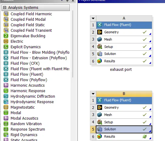
fig: setup.
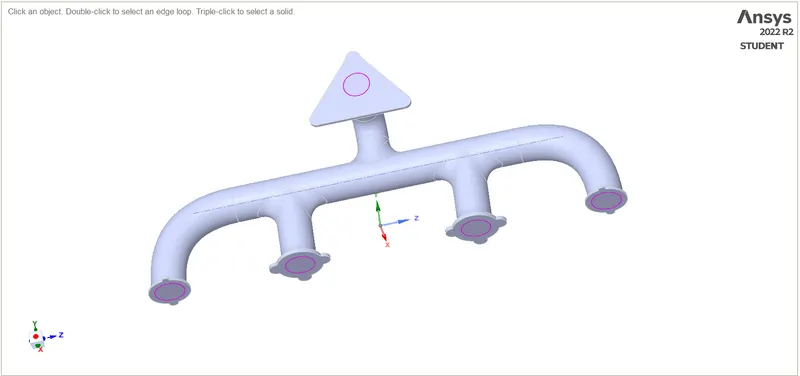
fig: raw model of the exhaust port.
2.Then i extracted the inner volume of the exhaust port by using the volume extraction option in the spaceclaim.
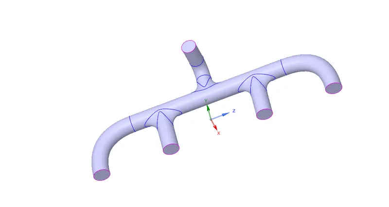
fig: extracted volume of the exhaust port
case 1 with inflation layers.
3. then i open the mesh part and started the meshing the geometry i have given the mesh size of 100mm.
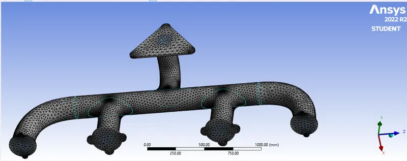
fig: meshed exhaust port.
4.then i went to the inflation layers meshing on the exhaust port. the inflation layers are made based on the first layer thickness with the y+ calculation.
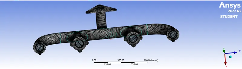
fig:exhaust port with the inflation layers.
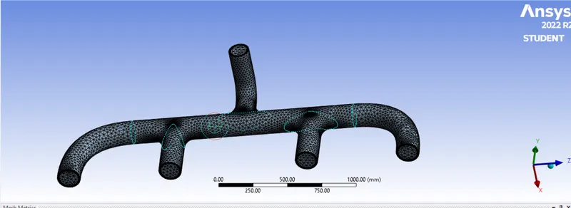
fig:inflation layers on the extracted volume.
5.for making the inflation layers i have selected the fluid domian i.e the fluid flow inthe volume only. the above fig is showing the inflation layers on the part.
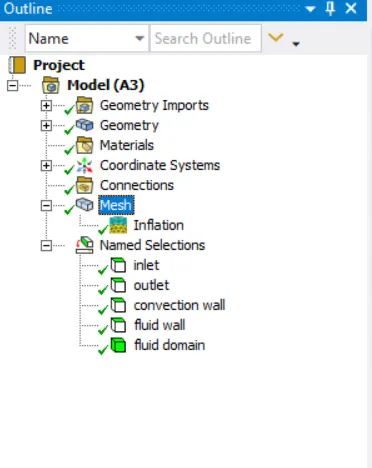
fig: mesh setup.
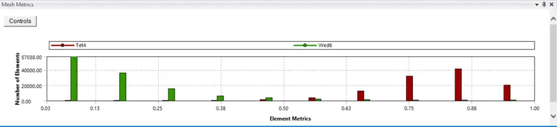
fig:mesh quality
6.then the meshing part is compeleted and i have given the names to the each part that is inlet, outlet ,fluid domain,convection wall and fluid wall.
CASE 2 without inflation layers
7.then i open the mesh part and started the meshing the geometry i have given the mesh size of 80mm.
fig: meshed exhaust port.
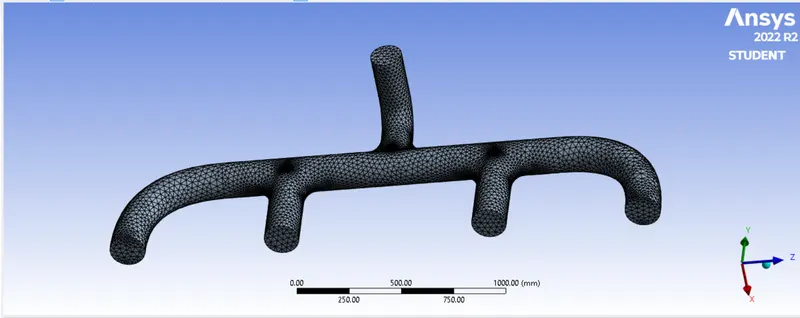
fig: fluid domain with mesh.
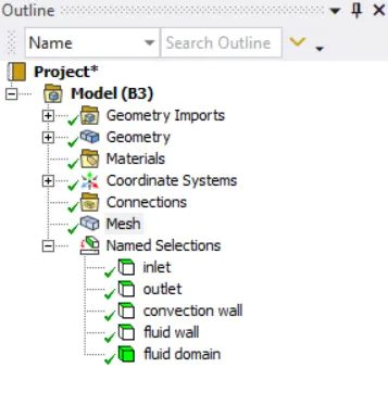
fig:mesh setup.
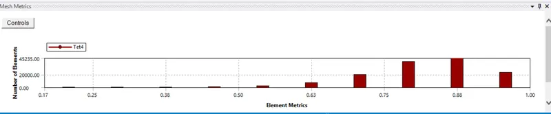
fig:mesh quality
8. then the meshing part is compeleted and i have given the names to the each part that is inlet, outlet ,fluid domain,convection wall and fluid wall.
SOLVER SETUP: it same for the two casess
9. then i open setup to give input to solve the simulation. here i have ON the energy equations , the k-omegha sst based solver. then i have went to the boundary conditions to give the input values inlet velocity 25m/s and inlet temperature 700k and the the heat transfer coefficent is 20 w/m2-k.
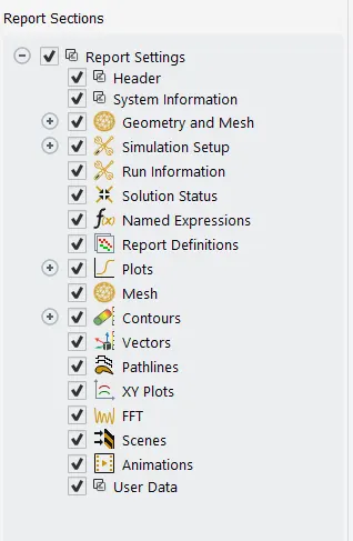
fig: solver condition setup.
10. then i have made report related to the wall flux under report definitions that is htc report. then i have made the contour plots for the temperature and velocity.
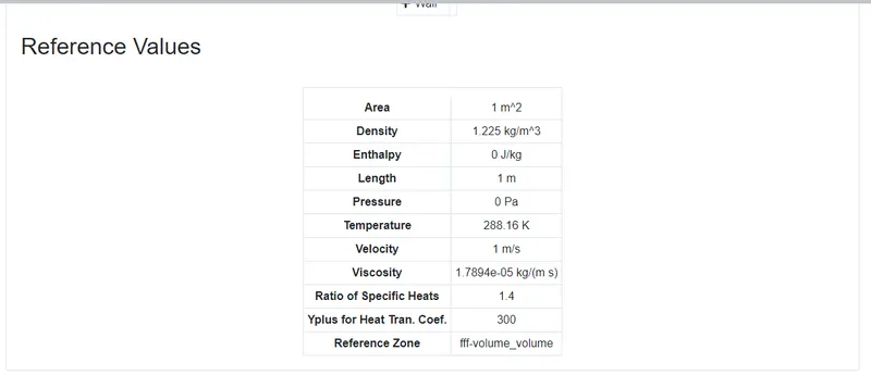
fig: reference values
CASE 1
1. the exhaust port with inflation layers
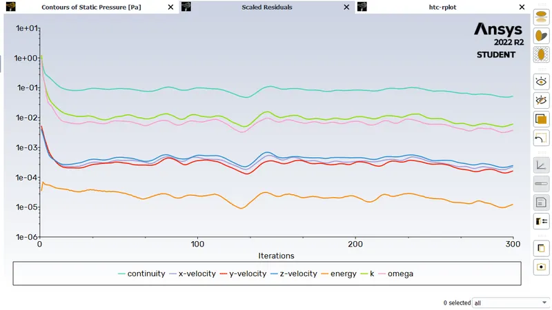
fig: Residual plot.
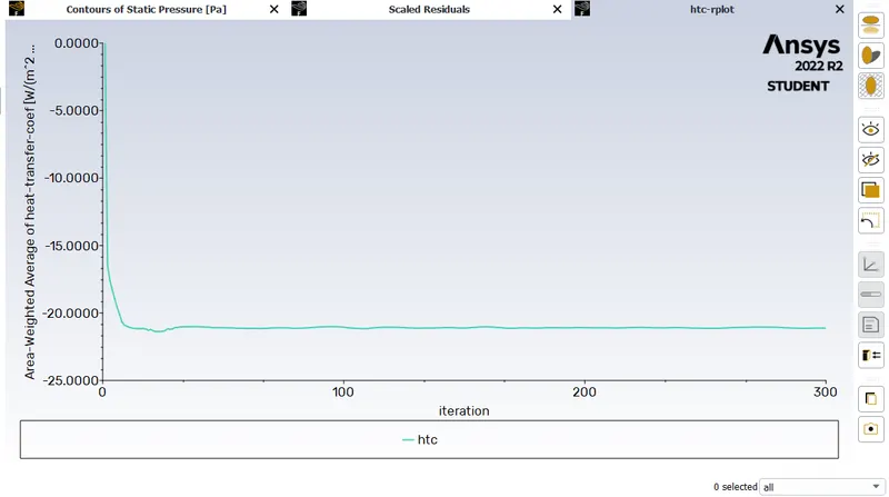
fig: htc plot.
OUTPUT:
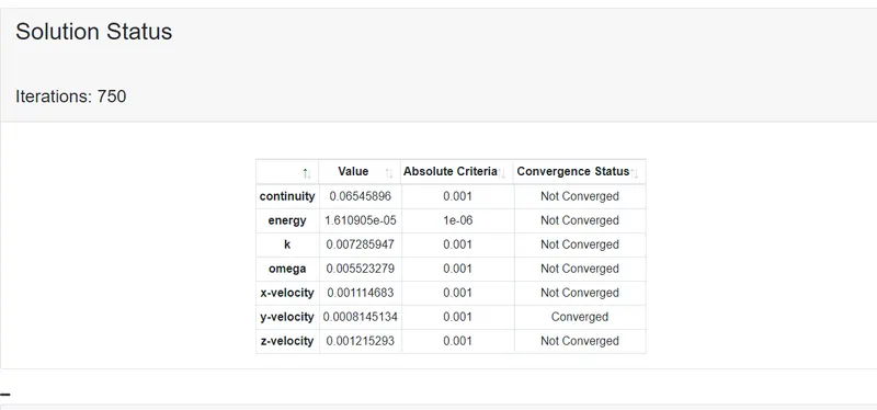
fig: converged and not converged values.
BUT here the value k,omega etc are some period of time coverged and then they are not converged.

fig: ouput of htc.
CASE 2 without inflation layers
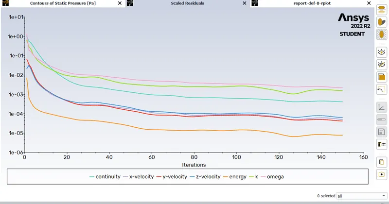
fig: Residual plot
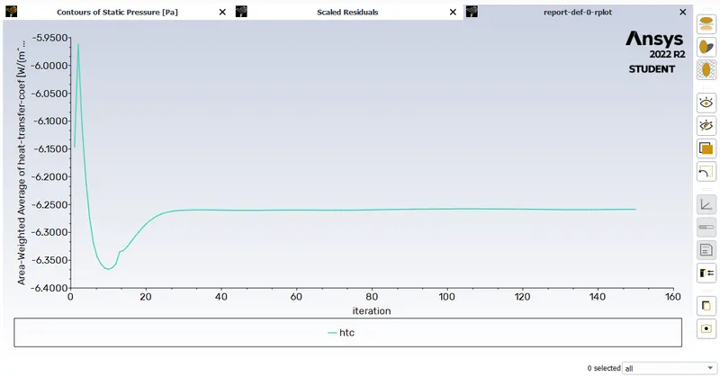
fig: htc plot.
OUTPUT:
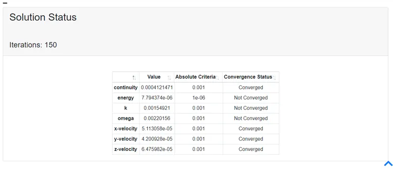
fig: converged and not converged values
here the values are converged for less no.of time steps.
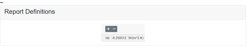
fig: output of htc.
RESULT:
case 1
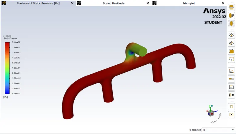
fig: pressure contour.
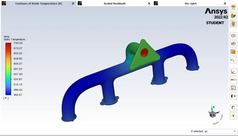
fig: temperature contour.
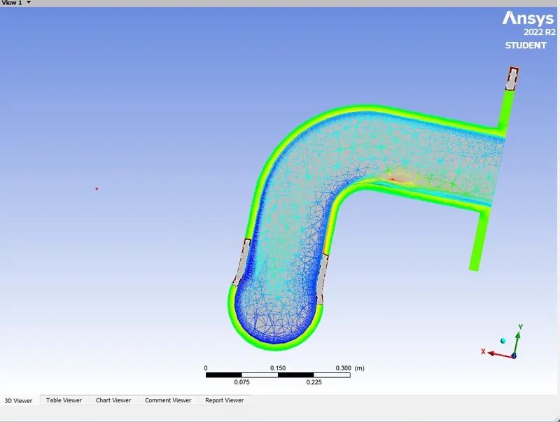
fig: turbulence kinetic energy of the exhaust port.
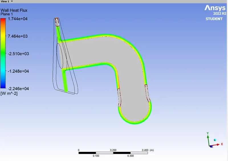
fig: wall heat flux of exhaust port
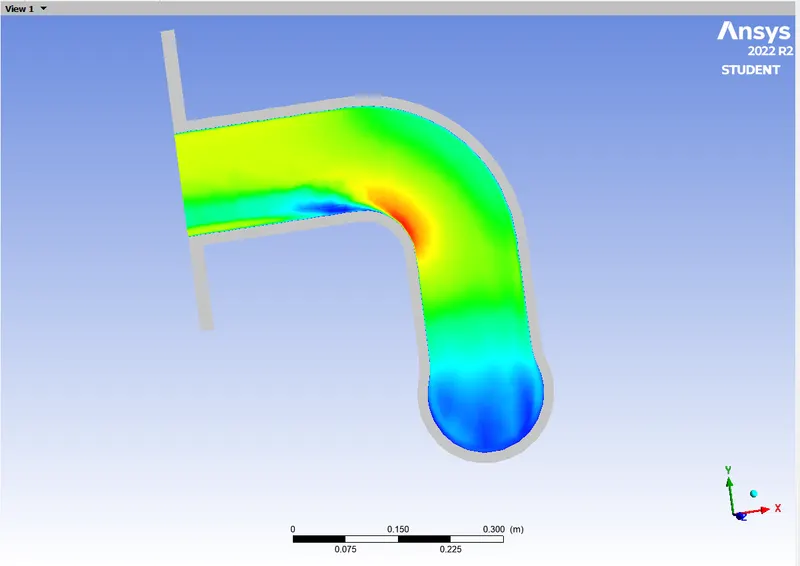
fig: velocity contour.
CASE 2
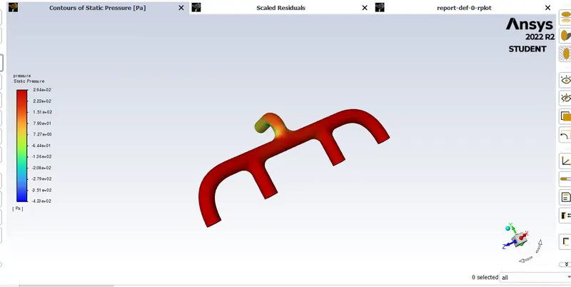
fig: pressure contour
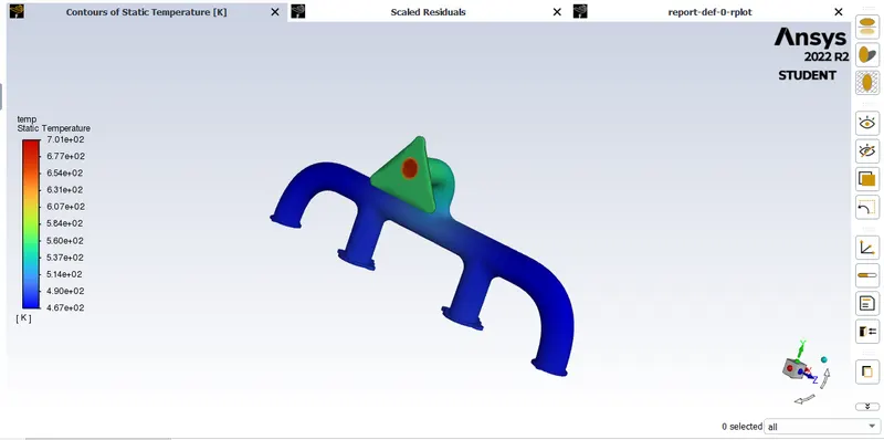
fig: temperature contour
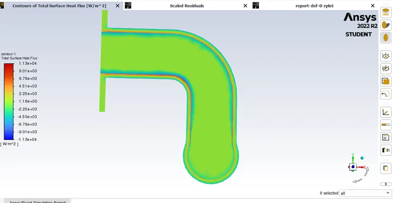
fig: surface heat flux.
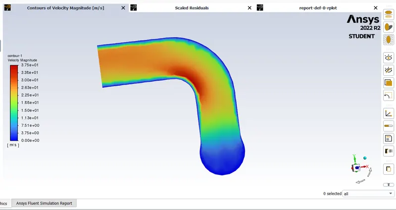
fig: velocity contour
CONCLUSION:
here i conclued that the result are more accurate in the first case as compared to the second case since it is refine mesh. the velocity is higher at the outlet of the port due the higher in temperature due to this reynolds numder is also high. but the both cases the htc value is small different i.e in decimals.
case 1 = -6.256302w/(m^2-k)
case 2 =-6.258512w/(m^2-k)
4Q:How would you verify if the HTC predictions from the simulations are right? On what factors does the accuracy of the prediction depend on?
By comparing with theortically calculating the nusselt number and to find heat transfer coefficient.
here the accuracy of the prediction depends on refine mesh, no.of inflation layers and number of elements. but it mainly depends on the pre process only