Week 4 - CHT Analysis on Exhaust port

Aim: To perform CHT Analysis on Exhaust port.

Objectives:

1. Give a brief description of why and where a CHT analysis is used.
2. Maintain the y+ value according to the turbulence model and justify the results.
3. Calculate the wall/surface heat transfer coefficient on the internal solid surface & show the velocity & temperature contours in appropriate areas.
4. How would you verify if the HTC predictions from the simulations are right? On what factors does the accuracy of the prediction depend on?

Conjugate Heat Transfer (CHT)

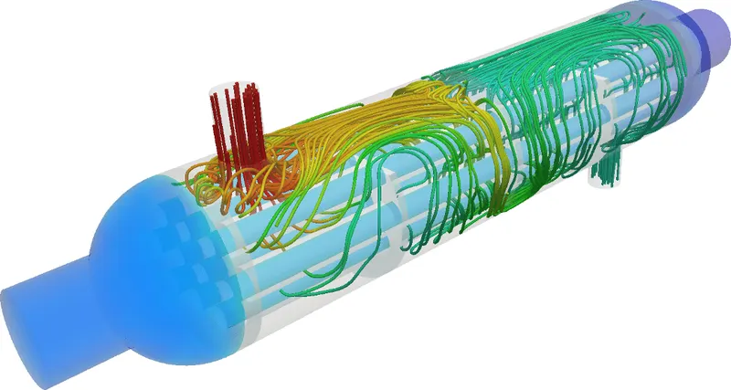
The Conjugate Heat Transfer (CHT) analysis type allows for the simulation of heat transfer between solid and fluid domains by exchanging thermal energy at the interfaces between them. Typical applications of this analysis type exist as, but are not limited to, the simulation of heat exchangers, cooling of electronic equipment, and general-purpose cooling and heating systems. This CHT analysis can be for this problem inorder to find the heat transfer from the fluid to the Solid exhaust port.

Simulation procedure:

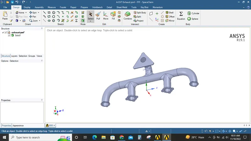
Exhaust port model is imported into the Space claim.

Topo checkup is performed to identify if there are any extra unwanted edges.

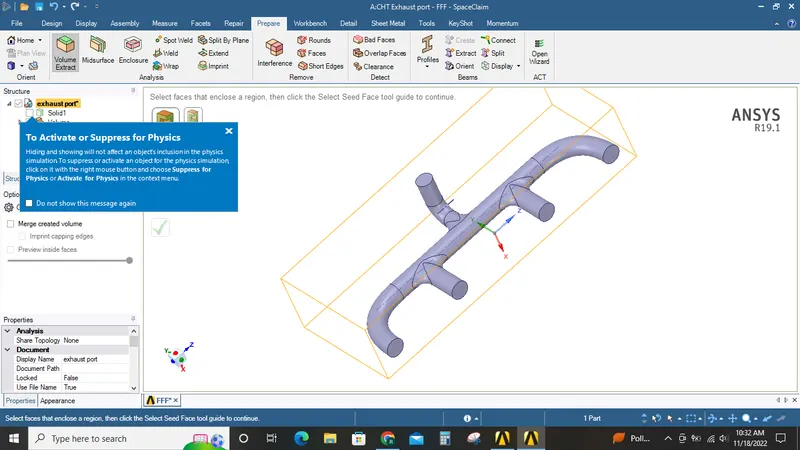
By using the volume extract tool fluid volume is extracted.

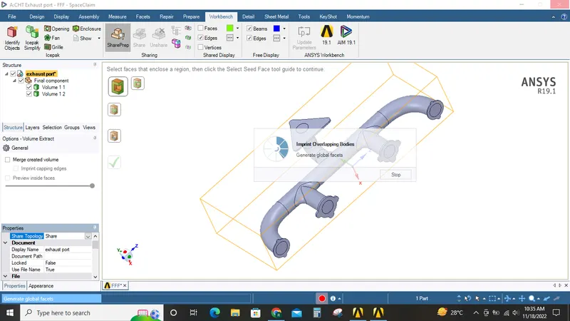
The fluid volume and Solid volume(Exhaust port) both moved to a new component.

The share topology property is set to share, this is done to enable the volumes to exhange informations between them.

Under the Workbench ribbon tab, share prep option is enabled.

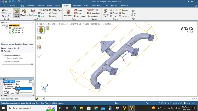
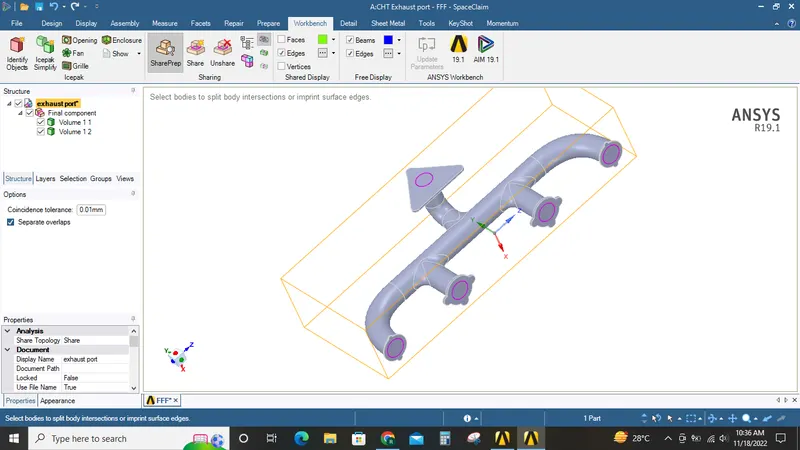
Now space claim is closed and Mesh module is opened.

The base mesh is created with default settings.

Now inorder to capture the physics near the walls of the exhaust port infaltion layer is added based on the Y+ value from calculation.

2. Justifying the value of y+ taken.

As we know the flow is turbulent, and we provide inflation layer near the wall , so basically we are focussing on the laminar region near the walls which is a part of the turbulent flow. In order to capture this small region, mesh sizing here should be small as well. To determine the size of the first cell from the wall (basically distance of wall surface to the cell node of the first layer of cell attached to wall), i.e. the y value we have the formula:

y+= yu*/v

y+=10 or less for cell node to be in the laminar region of the turbulent flow and >30 for cell node to be in turbulent region of the turbulent flow. Region between this is the transitional region.

Considering y+=10

V=5m/s

U*=frictional velocity where u*²=T/ρ

T=wall shear stress

Ρ=density=1.225kg/m³

Now, T= Cf*0.5*ρ*v²

Cf=friction coefficient=0.0576Re^-1/5

Re=ρDv/µ

D=0.166m (from space claim geometry data , we find inlet dia)

Ρ=density of air=1.225kg/m³

µ=Viscosity=1.7894e-05 kg/ms

v=5m/s

Re=56820.7

Cf=0.00644

T=0.0986 calculated from the above formula

Hence,

u*²=T/ρ

U*=0.283m/s

Hence, y=6.3mm from the formula

y+= yu*/v

Hence, any value below 6.3mm for inflation layer thickness is valid as it comes under the laminar region which is occurring near the wall(where we apply the inflation layer).

Inflation layer with total thickness of 6mm is used in this case.

Also the mesh of the solid volume is refined to 10mm.

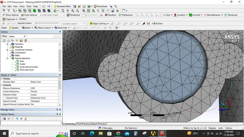
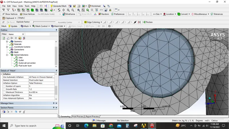
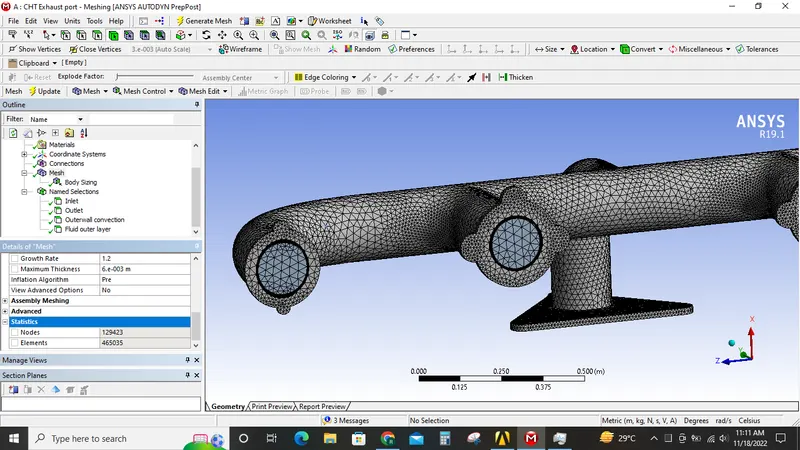
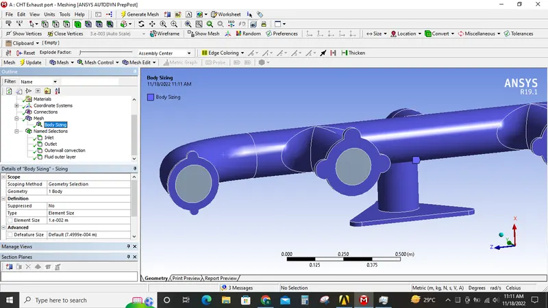
Now the mesh module is closed and Fluent is opened.

Mesh quality check is performed.

Under setting up physics steady state pressure based solver is used.

K-Epsilon with Energy model is used.

Under Boundary conditions the inlet velocity is set to 5m/s and temperature is to 700K.

Under materials Air is used as the fluid and for the solid volume aluminium is used.

Simulation is initilaized and run for 300 iterations.

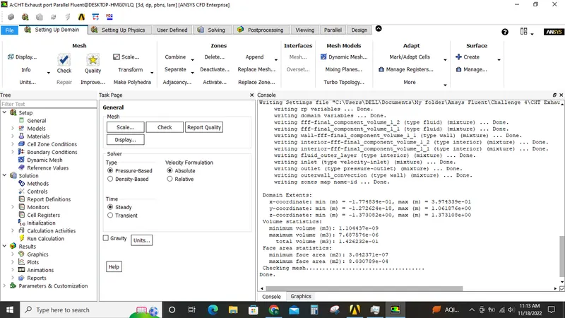
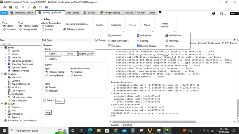
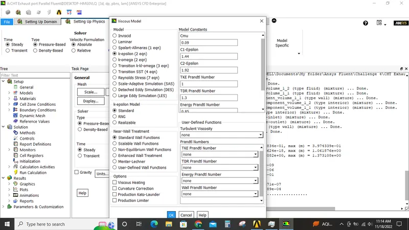
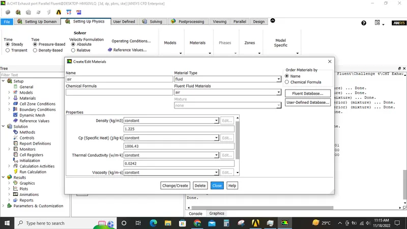
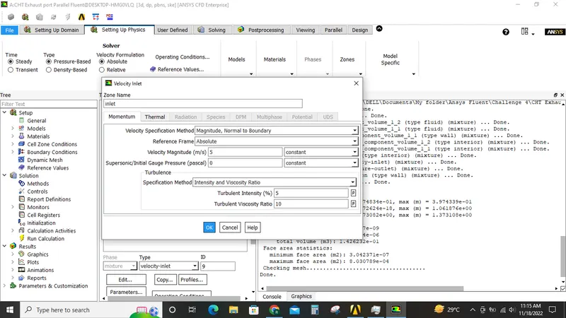
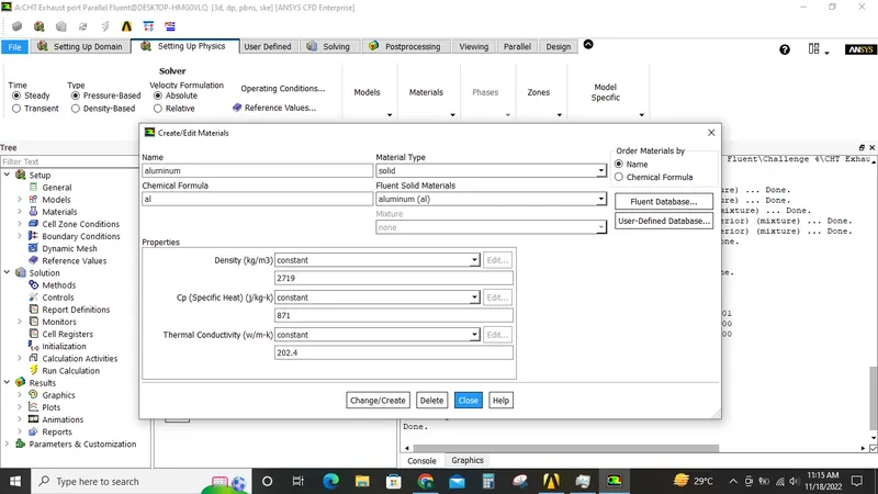
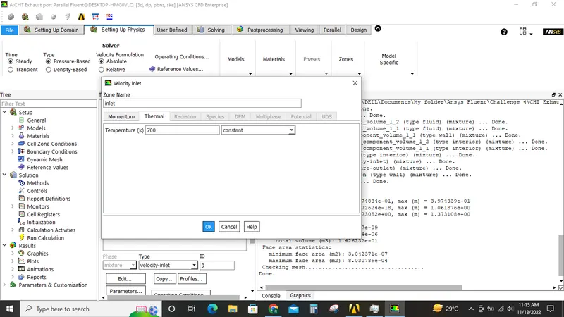
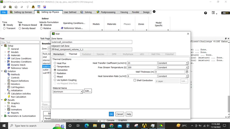
The results are shown below.

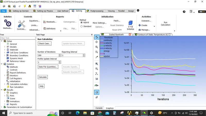
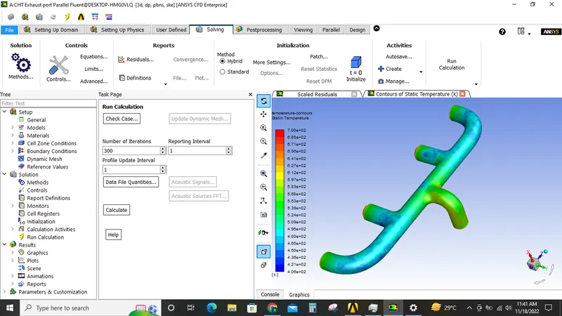
Now Fluent is closed and CFD post is opened.

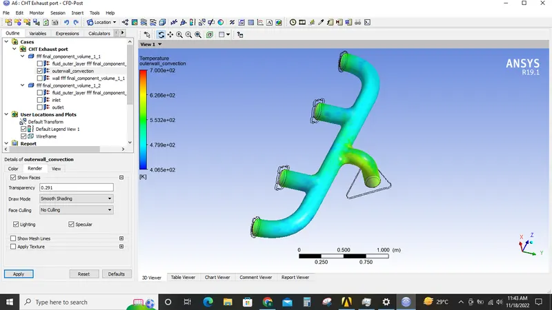
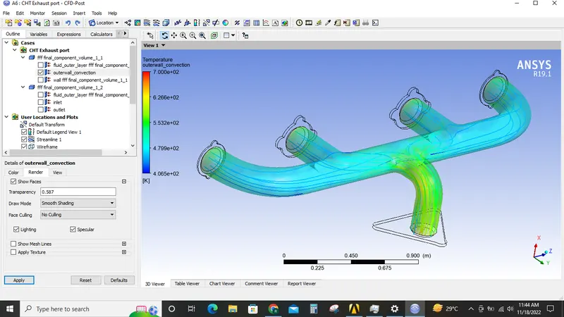
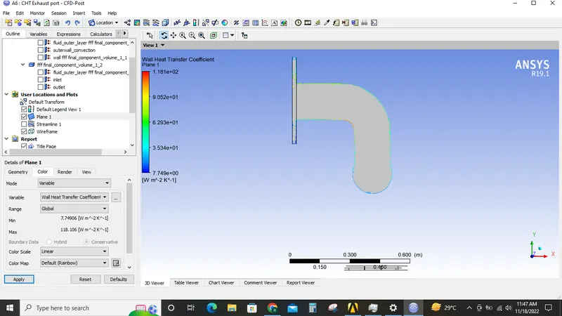
Temperature contours, stream line visualizations and Heat transfer contours on a plane in created in CFD post which are shown below.

Q3. Calculate heat transfer coefficient and show the temperature and velocity contours.

Creating a report>area weighted average>wall fluxes>surface transfer coefficient for inflation layer named selection.

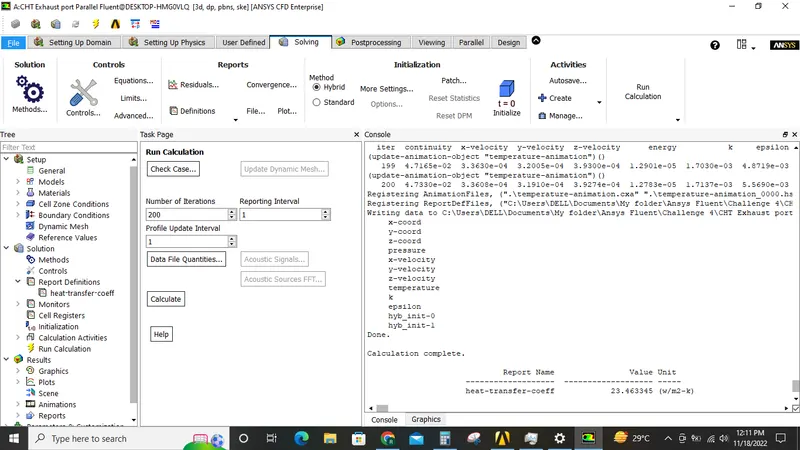
After running setup and computing heat transfer coefficient from the report. We get,

Heat transfer coefficient from Ansys fluent report: 23.46W/m2K

Q4. How do you verify if HTC Predictions are correct? On what factors does the accuracy of the prediction depend on?

Heat transfer coefficient from ansys fluent report: 31W/m2K

We verify value from the following relation:

Value from Dittus-Boelter correlation:

Nu=Nusselt number, Pr=Prandtyl number, Re=Reylond number

Nu=0.023Re^0.8 Prⁿ

n=0.4 for hot fluid

Valid for prandtyl no.( 7-160) and reylond number>10000,

Re=ρDv/µ

D=0.166m (from space claim geometry data , we find inlet dia)

Ρ=density of air=1.225kg/m³

µ=Viscosity=1.7894e-05 kg/ms

v=5m/s

Re=56820.7

This means the flow is turbulent, that’s why we used the turbulent model for simulation.

Pr=µCp/k

µ=Viscosity=1.7894e-05 kg/ms

k=Thermal conductivity=0.0242 W/mK

Cp=specific heat =1006.43J/kgK

Pr=0.744

Putting the two values of Re and Pr in Dittus-Boelter correlation:

Nu=129.9 i.e., 130

Nu=hL/k

k=Thermal conductivity=0.0242 W/mK

L=diameter of inlet =0.166m

h=heat transfer coefficient as per co-relation =18.9 W/m²K

Now the heat transfer coefficient value is more or less close to the vlaue obtained in the simulation.

Conclusion: We can see that the velocity at the outlet in greater than velocity at the inlet, this is because of mass conservation principle. Due to this higher velocity the temperature on the outer surface near the outlet is higher than the temperature near the inlets. Similarly heat transfer coefficient is higher near the outlet.

Ansys files are in the below link

https://drive.google.com/file/d/1jmVl7GVxU34mKn2A9ebu0hQlK0R_MWeS/view?usp=share_link