Week 4 - CHT Analysis on Exhaust port

Objective:

With regard to this obstacle,

• In the upcoming sections, we will provide a concise explanation of when and why a CHT analysis is performed.
• On an exhaust port, we will perform a simulation of both the flow of fluid and the heat transfer to the solid, also known as a CHT analysis.
• Then, we will present the velocity and temperature contours in the appropriate places after we have calculated the wall heat transfer coefficient on the interior solid surface.
• We will investigate whether or not the predictions made by HTC based on the simulations are accurate. Also include a discussion of the factors that will determine how accurate the prediction will be.

Conjugate Heat Transfer (CHT) analysis :

Using an analysis technique called "conjugate heat transfer," one may model the flow of heat from one domain (solid or fluid) to another (through conduction inside the solid and convection within the fluid) and back again. By simultaneously solving all of the pertinent processes involved in solid and flow field heat transfer, conjugate heat transfer analysis is able to properly forecast how heat will be transferred. The combination of heat transfer in solids and heat transfer in fluids is what's meant to be understood by the term "conjugate heat transfer." While convection typically takes the lead in fluids, conduction tends to be the dominant form of heat transfer in solids. It is possible to witness conjugate heat transfer in a variety of contexts, such as in the case of conduction through solids, free and forced convection in gases and fluids, and thermal radiation.

The three primary means by which heat is transferred are as follows:

The process of heat transfer that takes place when there is a temperature difference across a stationary medium is referred to as conduction. The process of heat transmission that occurs when there is a disparity in the temperatures of a surface and a fluid that is moving is referred to as convection.
The emission of energy in the form of electromagnetic waves is what we refer to as radiation (also known as thermal radiation). There is a positive net heat transfer by radiation between two surfaces that are different temperatures when there is no intervening medium in the path between them.

Conduction :

The transfer of heat energy through a solid or fluid occurs by a process known as conduction. This process is driven by the translational, rotational, and vibrational motion of atoms and molecules. Collisions between molecules are what transmit energy from highly energetic molecules to those with less energy. The higher the temperature, the more atomic and molecular mobility there will be. Conduction can take place in any medium, be it solid or liquid.In accordance with the Second Law of Thermodynamics, heat must invariably move from locations of greater temperature to those of lower temperature. When there is an issue with conduction, it frequently involves fluid flows at the boundary of the solid. These fluid flows act as a mechanism for either heating or cooling the solid. Because of the difference in temperature, energy can be transferred from more energetic particles of a substance to less energetic particles of that substance via interactions between the particles on molecular levels. This process is known as conduction. There is a correlation between the energy of random translational, internal rotational, and vibrational motions of gas molecules and the temperature at any given place in space.

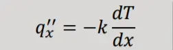
Energy is transferred from highly energetic molecules to less energetic molecules as a result of collisions between molecules. When there is a temperature gradient present, the transfer of energy always occurs in the direction of decreasing temperature. This is because larger molecular energies are associated with higher temperatures, and the transfer of energy always occurs in the direction of decreasing temperature. Because the molecules in liquids are closer together and their interactions with one another are greater and more frequent than in gases, the process of conduction is the same for liquids as it is for gases. When it comes to solids, conduction is linked to atomic activity that manifests itself as lattice vibrations. In the case of an electrical conductor, another factor that contributes to the movement of free electrons and the consequent transfer of energy is translational motion. The process of heat transfer can be quantified using the proper rate equations, which are then used to quantify the amount of energy that is being transported per unit of time. Fourier's law can be thought of as the rate equation for the process of heat conduction. This is represented mathematically for a one-dimensional plane wall as

In this context,

the rate of heat transfer per unit area in the x-direction is denoted by "q x" (W/m2)
k is the thermal conductivity, measured in W/mK, and it is a property of the material that makes up the wall.
The fact that the heat transfer is going in the opposite direction of the temperature gradient is denoted by the negative sign.

The process of convection:

Convection is the process of heat transfer that occurs when the bulk motion of a fluid is combined with the random molecule mobility of the fluid (diffusion). Conduction at the walls allows heat to be transmitted either into or out of the fluid. The fluid distributes the system's thermal energy to the various other components. Advection is the term used to describe heat transfer that occurs only as a result of the bulk motion of the fluid and does not involve diffusion.

There are three categories that convection heat transfer can be placed in:

Forced convection: Flow is produced by an external agent, such as a fan, a pump, or the natural winds in the environment.
The flow is produced by buoyant forces, which are caused by differences in density that are attributable to the temperature variations in the fluid. This type of convection is known as free (or natural) convection.
Convection can be either forced or natural, or both, if there are driving forces from the outside and buoyant forces within the system.
The concept that the rate of heat transmission is directly proportional to the temperature gap that exists between a fluid and a heated or cooled body is the foundation of the convection method of heat transfer.
Newton's Law of Cooling is the name given to this theory. The heat transfer coefficient, which is typically indicated by the symbol h, is the variable that determines the rate at which heat is transferred.

Here, 𝑞′′ = Convective heat flux
𝑇𝑠= Temperature of the solid surface
𝑇∞= Temperature of the fluid

The calculation of the heat transfer coefficient for a specific flow field is one of the most important aspects of the convection process.
The heat transfer coefficient is determined by the conditions that are present in the boundary layer. It is also influenced by the geometry of the surface, the characteristics of the fluid flow, and a number of other thermodynamic and transit characteristics of the fluid.

Transfer of Heat Via Radiation:

Producing heat via emitting radiation The emission of energy in the form of electromagnetic waves is what constitutes heat transfer. When heated above absolute zero, every particle of matter releases heat in the form of thermal radiation.
This emission occurs because of shifts in the electron configurations of the atoms or molecules, and electromagnetic waves are responsible for the transmission of the energy (or photons). The intensity of radiation is influenced both by the temperature of the body and the features of the surface. Radiation, on the other hand, does not rely on the presence of a material medium and can take place even in a vacuum. Conduction and convection are two more forms of heat transfer. At high temperatures, one of the most important ways heat is transferred is by radiation.
In addition to this, it is the only method of heat transfer that is possible in space, which is how solar energy is brought to Earth. The majority of applications mix heat transfer in solids and heat transfer in fluids to get their desired results. This occurs because to the fact that fluids can flow around solids or between solid walls, and also due to the fact that solids are typically submerged in a fluid. The analysis of temperature fields and heat transfer is made possible by providing a detailed description of the modes of heat transfer, the properties of the materials, the flow regimes, and the geometrical configurations. A description of this kind can also serve as the basis for a numerical simulation, which is a tool that can be used to forecast the effects of conjugate heat transfer or to test various configurations in order, for instance, to optimise the thermal performances of a particular application.

In the beginning...

• As the flow is travelling through the manifold, it is going to exchange heat with the solid; therefore, our goal is to replicate the process of heat exchange here. Our objective is to simulate the flow through it.
• We are going to accomplish this by initially presuming that the flow is coming through the exhaust, which is basically through all four inlets. Additionally, we are going to give or assume that the fluid is really very hot, and that is going to heat the solid pipe from the inside. Additionally, we are going to assume that there is a particular heat transfer on the external surface.
• Therefore, in a real-world scenario, as your engine is air cooled since it is exposed to air, and air that is close to the port has a particular heat transfer coefficient, and that would be provided as input, and the value of that coefficient depends on the external air reynolds number.
• We are able to simulate it in order to determine the value; however, in this case, all that is required of us is to provide the value itself, which is the heat transfer coefficient for the outer wall boundary condition.
• The next step is to begin the simulation by taking these presumptions into consideration.

PRE-PROCESSING AND SOLVER SETTING

CASE-I( MESH SIZE= 150MM)

Geometry

• When working with the fluent module, we need to open spaceClaim and import the geometry.
• If you examine the geometry very carefully, you'll notice that it has a solid portion.
• 
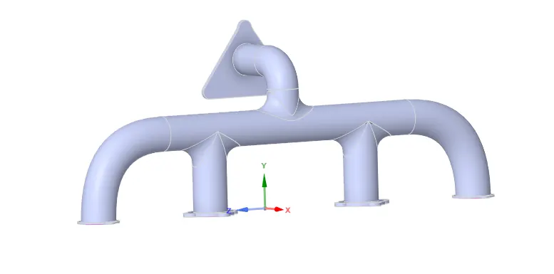
• Therefore, the first step is to determine the volume of the fluid.
• Because of this, we are required to go to,
• preparation -> volume extract -> select edge selection -> then select all of the edges of inlet and outlet -> then hit ok when you're finished.
• It is anticipated that a volume of fluid will be produced.
• 
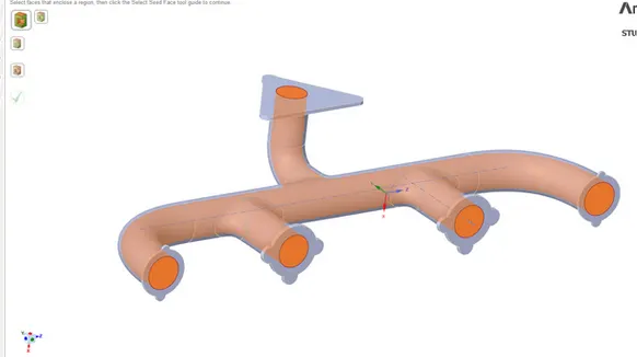
• We should have both of the volume perfectly overlap, and in order to do that, we need to share the topology of our meshes. For the CHT simulation.
• 
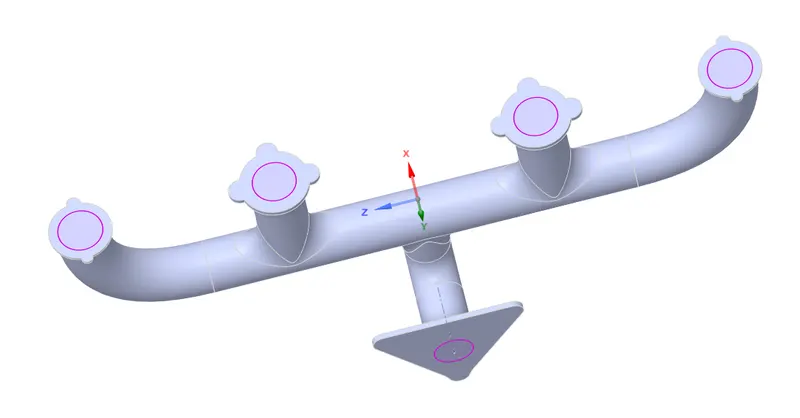
• When the sharing is finished, the area that has been shared will show in purple, as shown above.

Meshing :

• 
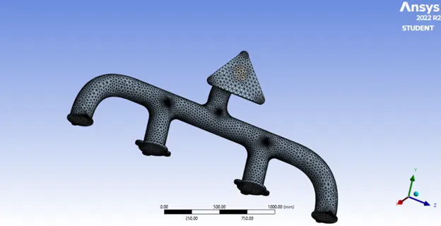
• In order to mesh our model, we first open the Mesh tool, which allows us to mesh it and then utilise it to solve our model.
• Before beginning the meshing process, it is best practise to give each of the surfaces a name. So, let's go ahead and do it.
• We begin by selecting the entity through the use of the entity selection through the use of faces in order to create a name for our entity selection.
• 
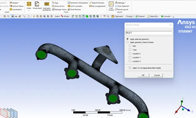
• steps: using the edge selection tool, select the edge you wish to name; next press the N key; finally, give the selection a name.
• You can see additional walls like flangs that have not been selected, and you can name them if you want to. However, even if you don't name them, ANSYS mesher will still automatically import those into fluent as a wall by using the deflection method. This is because we are going to use convective BC for it. In the same way, we name our inlets, outlets, and for outer face just double click on the outer part any where and ANSYS mesher will

• 
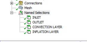
• Then the following step is to mesh the materials.
• We begin by developing our base line mesh by selecting the mesh option located in the side panel.
• Next, we will refine the mesh.
• Let's combine all of the geometries into one.
• As soon as the mesh is finished, we will need to determine what aspects need to be improved upon.
• Let's go through each step in order.
• First things first, let's get the inflation layer set up.

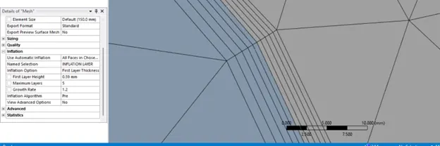
a) Inflation:

With the help of the inflation layer, we were able to design a mesh that was body-fitted.

• This indicates that it produces a layer of mesh that is identical to the geometry.
• Because the flow at the interface is really critical, and because we want to compute the heat transfer at that location, we need to take that region and build inflation layers. This will ensure that the flow is captured properly, and that the values are calculated exactly.
• In order to accomplish this, we will begin by picking the fluid component and renaming it as the inflation layer.
• In the global mesh editor, choose the inflation option. Then, in the section labelled "use automatic inflation," choose all of the faces in the named selection you've chosen. Finally, in the section labelled "named selection," choose the inflation layer that you've just named.
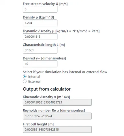
• In addition, for the inflation option, the first layer thickness is what we use, and we determine it based on the y+ value and the turbulence model that we employ.
• Because we are working with the k-omega SST turbulence model here, the value of y+ should fall between between 0.1 and 5.

• Inflation layer being added in accordance with the Y+ model.

  The Y+ model is computed with the Y+ calculator.

• 
• 

Problem Setup :

• In order to prepare for our problem, we launch Fluent and configure the initial conditions, boundary conditions, material, and so on.
• First things first, we do a quality check on the mesh by using the perform mesh check under domain command.
• If there is no indication of an error in the console window, then we are free to move on.
• The next step is to configure the physics, during which we make choices about the solver, viscous model, beginning and boundary conditions, and so on.
• In order to solve our model, we make use of a pressure-based solver that operates in a steady state.

Physics :

General :

Solver type : pressure based

time : steady state

velocity formulation : absolute

models :

viscous model : k-omega SST

Material : Fluid : Air

Solid : aluminum

Inlet :

velocity : 5 m/sec

temperature : 700K

Outer wall convection :

type : wall

Theremal conditions => convection : Heat transfer coefficient = 20 W/m^2 K

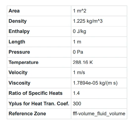
start initilize

Result for Case-I

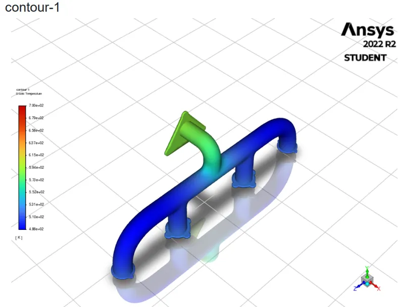
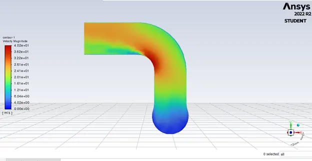
Temperature contour, volume rendering,Body

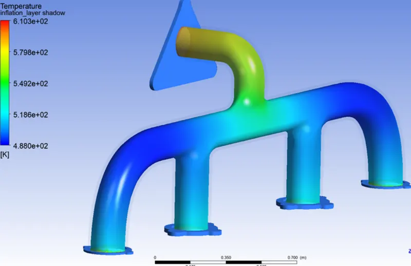
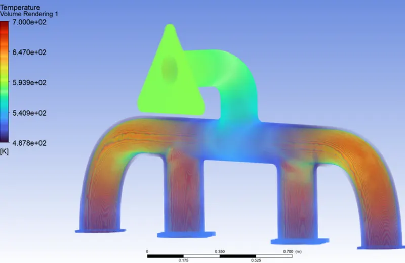
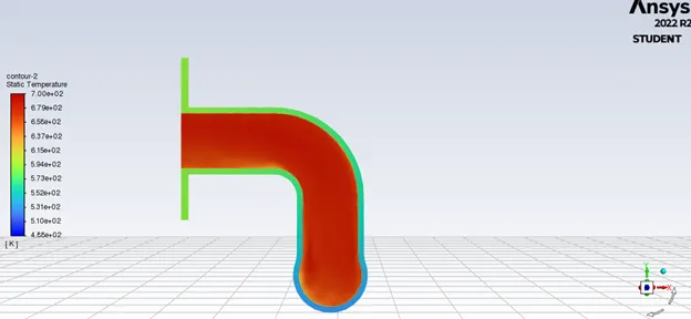
The colour near the wall depicts the heat transfer that occurs as a result of convection, and the temperature of the pipe is affected by the temperature of the fluid in the pipe.

CASE-II( Mesh = 17mm)

Meshing length is changed to 17mm and mesh is generated

• 

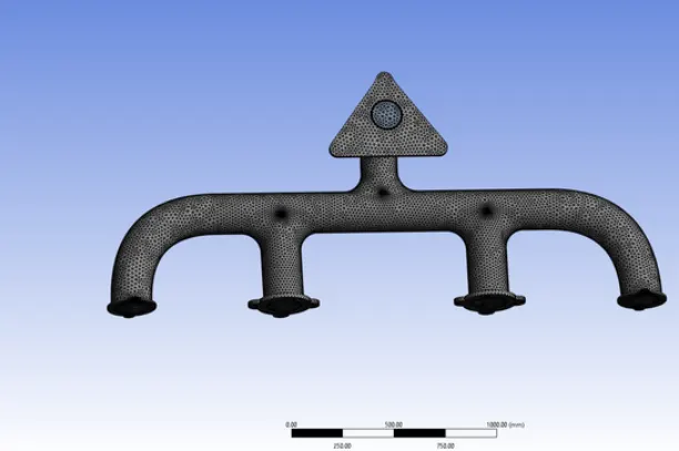
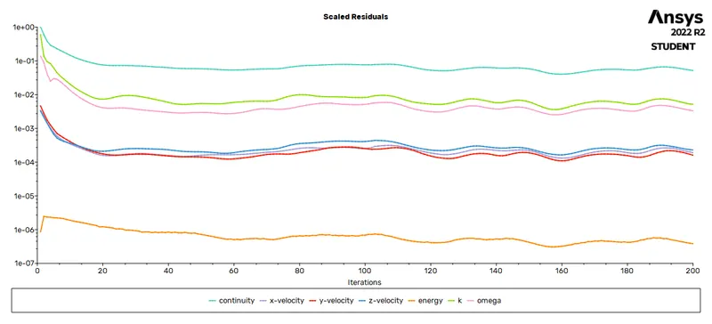
Results Case-II

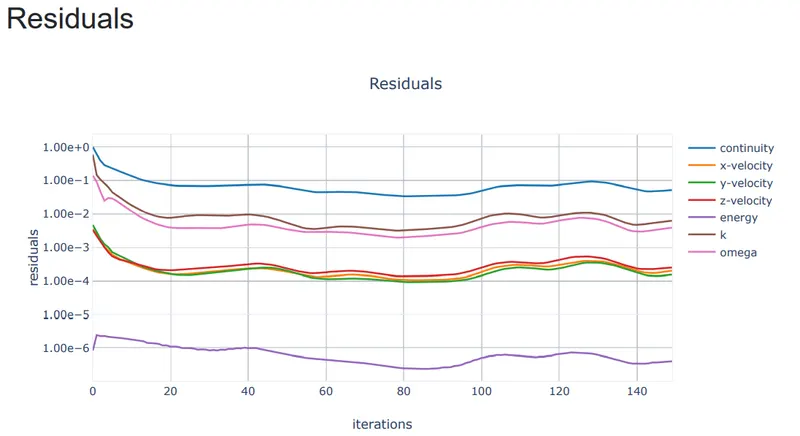
Residual plot

• 
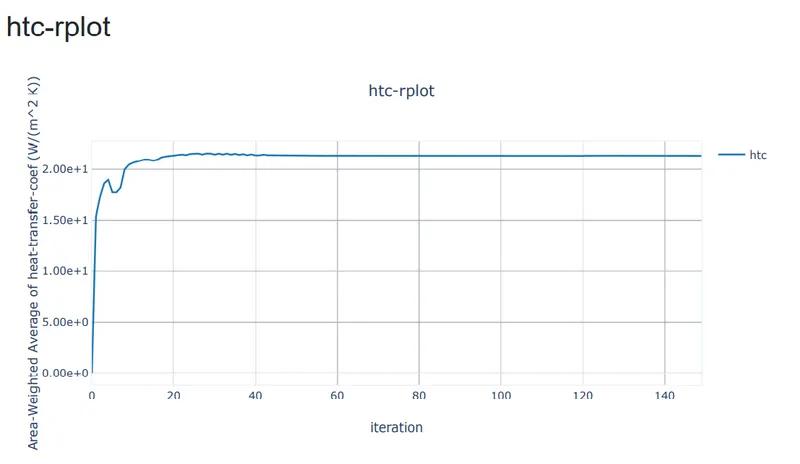
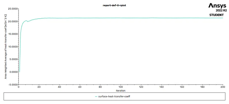
• htc plot
  
  

Contours:

• 
• 
• 
• 
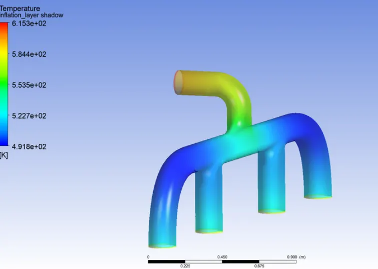
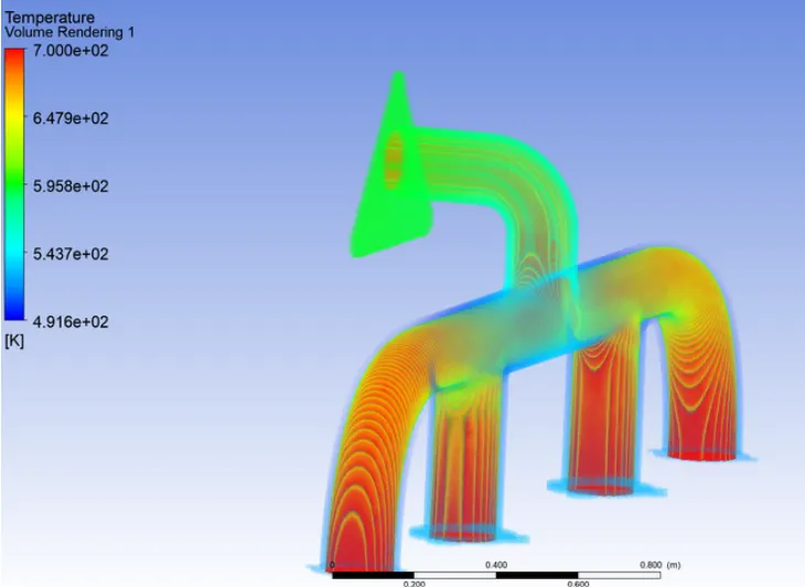
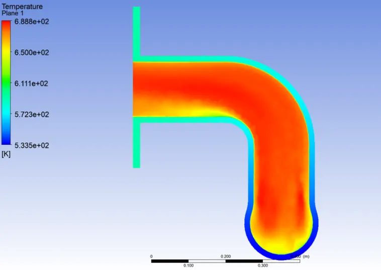
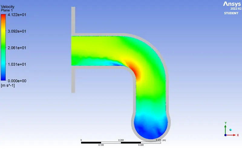
• Surface heat transfer
• 
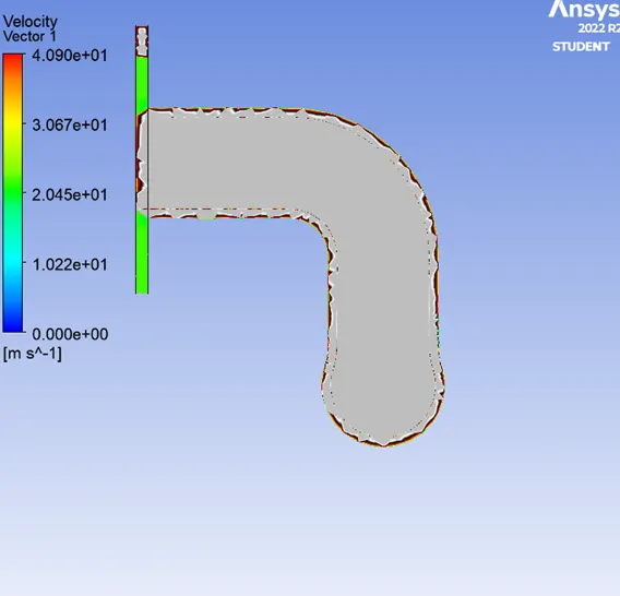
• The wall surface displays both the heat transfer coefficient and the changes caused by the presence of hot fluid.

COMPARISSION

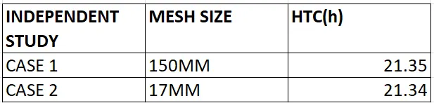
In general, the results were more sensitive to the grid size than they were in this situation, thus the degree to which they changed was limited. However, the results did improve with decreasing mesh size. If we dropped the mesh size much further, the results would vary even more; however, we are unable to do so because the student edition only permits 5 million elements.

Analytical Heat transfer coefficient

Conductivity(k)= 0.0242
Cp= 1006.43
Density= 1.225
Diameter(D)= 0.166
Reynolds number(Re) = 55119.8
Prandtl number(Pr)= 0.79

Nu(nusselt number)= `(h*D)/K`

Nu= `0.023*Re^0.8*Pr^0.3`

h= 20.1

`he analytical data for the heat transfer coefficient is 20.1 and the data of the solver is 21.34, hence the result is quite close to being accurate`

Conclusions

• An effective CHT study of the exhaust port was simulated in ANSYS _FLUENT.
• As can be seen in the comparison between the result and the analytical data, the result is quite close to being accurate.
• It's possible that if we expand and enhance the Grid, it will become more useful. We have the potential to produce even more impressive outcomes.
• Although decreasing the mesh size from 150 millimetres to 17 millimetres helped improve the results, this just demonstrates the necessity for an even finer mesh size if a better solution is to be found.
• Unlike the k-epsillon solver, which is optimised for outlet flow, the K-omega solver produces accurate results since it is more suited to Wall-based solution.

Factors influenced Accuracy

• We need to ensure that share topology is set to share because this affects the accuracy of the prediction.
• Only then can the meshing be consistent and fully connected.
• An appropriate turbulence model must be chosen.
• Since the flow is confined by walls, the k-omega SST will work exceptionally well.
• The precise Y+ value is also crucial when choosing the turbulence model.
• In the workbench, we need to allow share(share prep) by clicking share.
• If you skip this crucial step, you won't be able to observe the unique connection between them.
• This procedure takes care of the interface creation, so that there will be a single interface between the solid volume/block and the fluid volume/block.
• For the boundary, a precise heat transfer coefficient is required.
• Only then do we arrive at a complete and correct answer.
• If the numbers you're providing have decimal places, like those for inflation layers, be sure to include those decimal places.
• Since the heat transfer at the interface is crucially vital to determine, it is necessary to isolate that area and inflate the layers there to ensure accurate flow collection and value determination.