Week 4 - CHT Analysis on Exhaust port

Week 4 - CHT Analysis on Exhaust port.

Aim:

To simulate an internal flow of hot air in the exhaust port and study for the Conjugate heat transfer in the simulation, to perform mesh independent study and compare the results.

Introduction:

CHT Analysis means Conjugate Heat Transfer, modes of heat transfer are generally conduction convection and radiation. Conduction is observed within same kind of molecules (within a solid), convection occurs between different kind of molecules where bulk motion is involved (between solid and fluid). Any situation where both conduction and convection can co-exist within a system, then it is called as Conjugate heat transfer. Though conduction and convection co-exist either one can be dominating over the other, that is given by a non dimensional number called Nusselt number.

Here, when hot air is flowing inside the exhaust manifold, the mode of heat transfer between the hot air and the exhaust manifold inner wall is convection, and within the walls of the exhaust manifold is conduction. Finally, between the exhaust manifold outer walls and the ambient air is again convection.

Solving and Modeling approach:

We shall solve for 2 cases as discussed in Aim.We will be using ANSYS Fluent solver to create the geometry and perform unstructured tetra CFD mesh with boundary definitions, setup the physics of fluid flow and run the iterations to get solutions, using post processing to interpret the data in form of plots,contours, vectors, streamlines etc.,

With velocity of 5 m/s and k-omega SST model we shall study grid independence for CHT analysis of exhaust port with RANS. When we say grid independence study we shall study for 2 cases as follows.

Case	Baseline element size (mm)	Inflation layer element size (mm)
Case 1	150	150
Case 2	50	20

We shall keep in mind we are using a student version of ASNYS, so we are limited with the number of elements to play with. Then, we tabulate the case study results and compare it with the open literature or book data results to validate the simulation.

Preprocessing and Solver setting:

Let us open ANSYS workbench, now opening Fluent flow can be done by drag and drop in the schematic window or by double clicking on Fluent. The fluent workflow is in a series of steps such as GEOMETRY > MESH > SETUP > SOLUTION > RESULTS. Each step has to be completed for the next step to initialize.

In the grid independence study we shall consider case 1 and discuss in detail,

GEOMETRY >

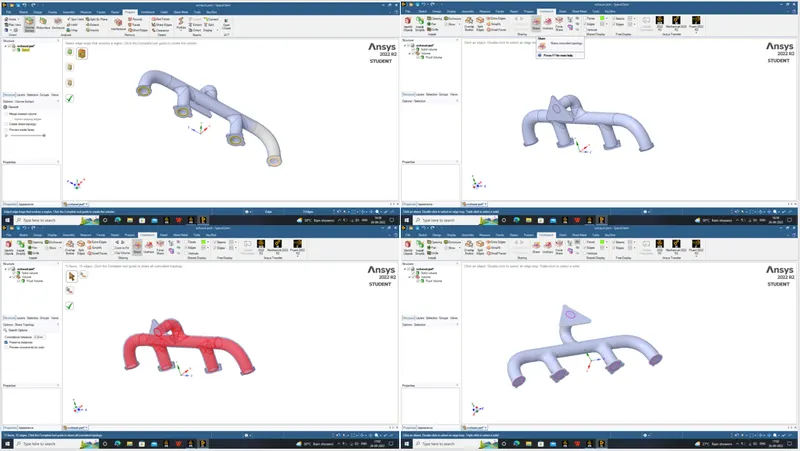
In the Fluent, right click on the Geometry and select New SpaceClaim Geometry. The space claim application opens, select FILE > OPEN and open the Exhaust port model.

We can check for geometry error using the EXTRA EDGES tool under PREPARE.

For flow study we need Flow domain, we shall create one using VOLUME EXTRACT option. Using the select edge we can select the inlet and outlet edges to create a fluid volume. We can rename our existing solid and fluid volumes for ease of identification and use in the simulation. After which, we need to perform SHARE TOPOLOGY so that there is interaction of nodes between the fluid volume and the solid volume.

We are good to go now. Once the geometry is ready, we can close space claim and check that the fluid flow (fluent) geometry is updated indicated by a green tick.

MESH >

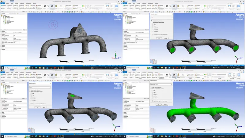
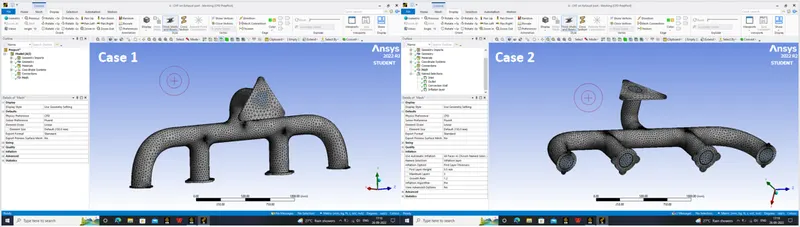
Right clicking on the Mesh and selecting edit opens the Mesh window. Mesh window is preloaded with the geometry we have worked on earlier, so clicking on the GENERATE MESH should create a mesh automatically.

We shall use INFLATION layers for the fluid volume outer surface with 0.5 mm as first layer thickness with 6 layers and 1.2 as growth factor. Since we already used share topology option, the mesh should look good.

For case 2, we shall use MESH > INSERT > SIZING and input size as 20 mm for inflation layer and the base mesh size shall be 50 mm.

Any changes made, click on the update icon to update the mesh details or else there is an indication of a thunderbolt sign asking the user to update.

We shall name the entry and exit surfaces such as Inlet, Outlet, Wall by selecting the outer faces and using the ‘N’ button and name them as Convection wall. We shall select the fluid volume outer surface and name it as inflation layer. Once this is done, we should see a green tick near Mesh. we can close the mesh window.

SETUP >

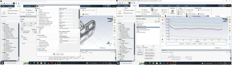
Right clicking on the Setup, opens the Fluent launcher. In the Fluent launcher select 3D, Double precision and select the number of cores as per the user system configuration and click on start.

Upon opening, there are some selections to be done to define the simulation definitions, we shall select Type: Pressure based, Velocity Formulation: Absolute, Time: Steady. Under the Physics tab, we can turn on viscous and select k-omega > SST as well. Turn on Energy. Method is Coupled method.

Under the materials we shall select air as our default material with material type as fluid. since we are dealing with the CHT analysis, we shall consider the solid volume also with aluminium as the default solid material.

Under the cell zone conditions, select the solid volume and check for material selection is solid, and fluid material for fluid volume.

We can proceed to define boundary conditions, as follows

Inlet : velocity magnitude = 5 m/s , Temperature = 700 K

Outlet should be a pressure outlet. For the convection wall, we can input heat transfer coefficient as 20 W/m^2 K.

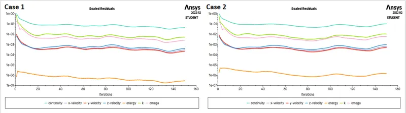
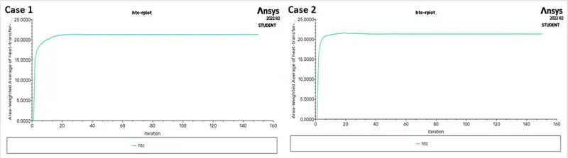
For generating surface reports, click on the Solution > Reports > Definitions > New > Surface Report > Area weighted average > Wall fluxes > Surface heat transfer coefficient for the heat transfer coefficient in the inflation layer. Now, it's time to start the simulation. In order to start the simulation for the above set up physics, we need to initialize the entire flow field by clicking on the t=0 initialize icon. In the Run Calculation we can input the number of iterations to be run (in this case 150) and clicking on the Calculate should start the iterations. After iterations, we get scaled residuals, average temperature plot and standard deviation plots.

We need velocity and temperature contours as well, to get them we can create a transverse cut plane i.e, XY plane and make new contour in Results > Graphics > Contours > New temperature for temperature contour and velocity for velocity contour. The scale can be edited by double clicking on it.

In the Outline view under Simulation Reports, clicking on the Report Outline > Generate should generate a Ansys Fluent Simulation Report which is automatically generated with all the information of the simulation in it. This can be exported as a PDF also. We are done with setup, we can close the setup.

SOLUTION >

Since some solution is calculated in the setup itself, we can see the green ticks in both setup and solution too.

RESULTS >

Right clicking on the Results should open the Post processor. Default view is a wireframe model, we can create a plane in XY and in YZ to view contours and vectors. Selecting the Vector and selecting the plane creates a velocity vector.

Similar to setup and solution, all contours and plots can be created here, in addition to that we can create an animation of the velocity contour by clicking on AUTOSAVE during the solution and clicking on ANIMATE select make movie and save in desired location.

For Case 2, we shall repeat the same except for changing the grid size in meshing step. We can simply DUPLICATE case 1 fluent file and edit in it.

RESULTS:

After repeating the similar manner of simulation procedures for all cases from aim, we have a handful of data to compare and study. We shall put in order all the contours, plots and vectors for us to compare and come to a conclusion. Here, only the results of all cases are displayed, its inference and interpretation shall be discussed briefly in conclusion.

Scaled Residuals

Surface heat transfer coefficient plot

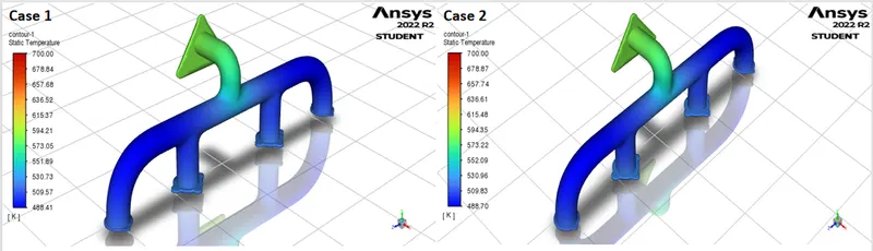
Temperature contour

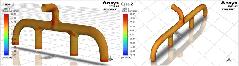
Surface heat transfer coefficient contour

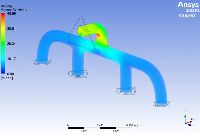
Volume rendered Velocity contour (Case 1)

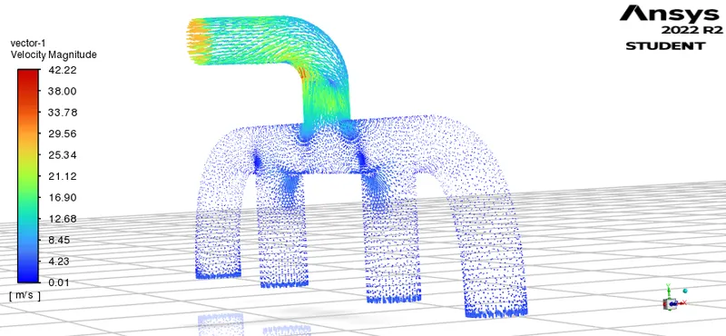
Velocity vector (case 1)

CONCLUSION:

From the results of all 2 cases, let us tabulate for surface heat transfer coefficient with respective grid sizes.

Grid Size	Case 1	Case 2
Baseline mesh	150	50
Inflation layer mesh	50	20
No.of elements	242887	315714
Surface heat transfer coefficient	21.32	21.34

Analytical solution and validation:

Reynolds number for the given flow of 5 m/s with 0.16 m as diameter for air at ambient temperature is 56820. which indicates the flow is turbulent in nature. From the Dittus Bolter heat transfer coefficient relation,

from the HMT data book, and Prantl number from data book is 0.71. solving for the equation with the Prantl number from data book, we get 21.5 W/m^2 K as the heat transfer coefficient.

INFERENCES:

From the grid independency study, we come to know that the finer and coarse mesh gives similar results. We have obtained (21.3 W/m^2 K ) the expected heat transfer coefficient close to 21.5 W/m^2 K.

As the finer size mesh elements doesn’t affect the surface heat transfer coefficient, maybe the velocity change can affect the output result, which again is another case study by itself.

From the temperature contours, we can see that the average temperature is around 500 K. and Velocity contours shows wake areas at the bends.

Also, velocity at the outlet is high compared to other areas because of conservation of mass flow rate at the outlet, since flow rate of 4 inlets add up in the outlet.

The surface heat transfer coefficient is higher at the bends and the inlet area, to be more specific in observation wherver the velocity is low there is increased surface heat transfer.

References:

International Journal of Engineering and Advanced Technology (IJEAT)
ISSN: 2249 – 8958, Volume-6 Issue-5, June 2017
79
Published By:
Blue Eyes Intelligence Engineering
& Sciences Publication Pvt. Ltd.
Numerical Study of Exhaust Manifold using
Conjugate Heat Transfer
Sagar G. Rautrao, Bhagwan R. Shinde