Week 4 - CHT Analysis on Exhaust port
Aim
To perform a Conjugate Heat Transfer analysis of the given Exhaust port to visualise the temperature and velocity inside. Further, estimate the Heat Transfer coefficient and validate the same.
Introduction
Conjugate Heat Transfer (CHT) comprises heat transfer in solids, dominated by conduction, and heat transfer in fluids, dominated by convection. The processes are divided into two subdomains and are calculated separately using their respective governing equations. Conditions at the interface of the two are then used to determine the distribution of the temperature/ heat-flux. Conjugate heat transfer analyses are quite often used in HVAC systems, heat sinks, engine cooling, etc.
Method
Geometry and Fluid/Solid domain
The geometry of the exhaust port was provided and shown in the image below. It contains five inlet ports and one outlet port and is enclosed by a casing made of aluminium.
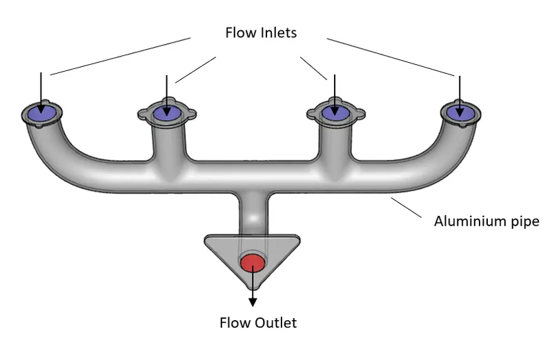
Pre-processing of the geometry was performed using Spaceclaim, where the extra edges were removed and the internal fluid volume was extracted. Finally, the fluid volume and the solid volume of the casing were made to share topologies in order to obtain a coherent mesh for simulation.
Mesh generation
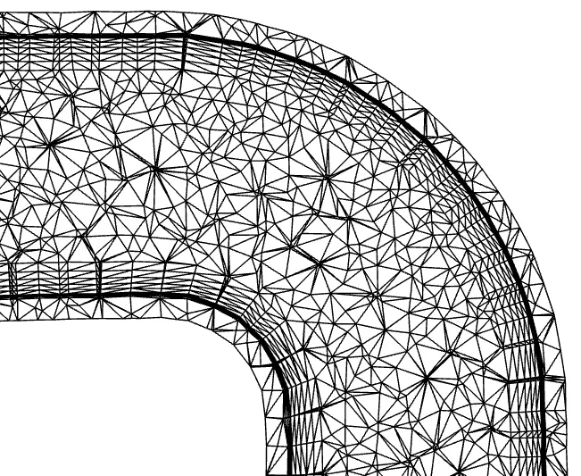
An initial baseline mesh was generated followed by a refined mesh to analyse the exhaust port. For both cases, four layers of inflation layers were generated in the fluid volume and two layers were generated in the solid volume.
Baseline:
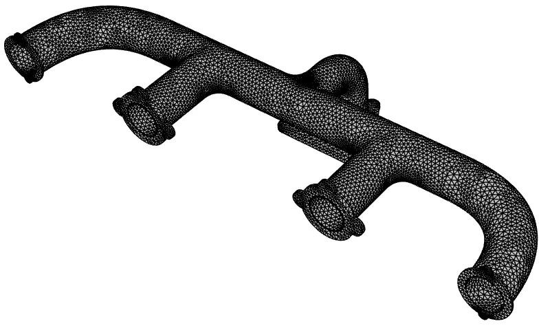
The baseline mesh was generated with an element sizing of 2.8e-2 m for both the solid volume and fluid volumes. An edge sizing of 2e-2 m was implemented on the inlets and outlet edges to capture their curvature properly. The resulting baseline mesh was generated with 280k cells and can be seen below:
Refined:
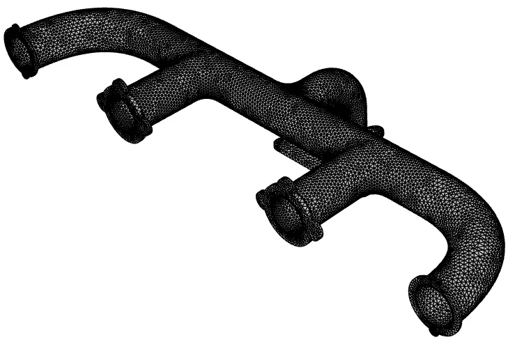
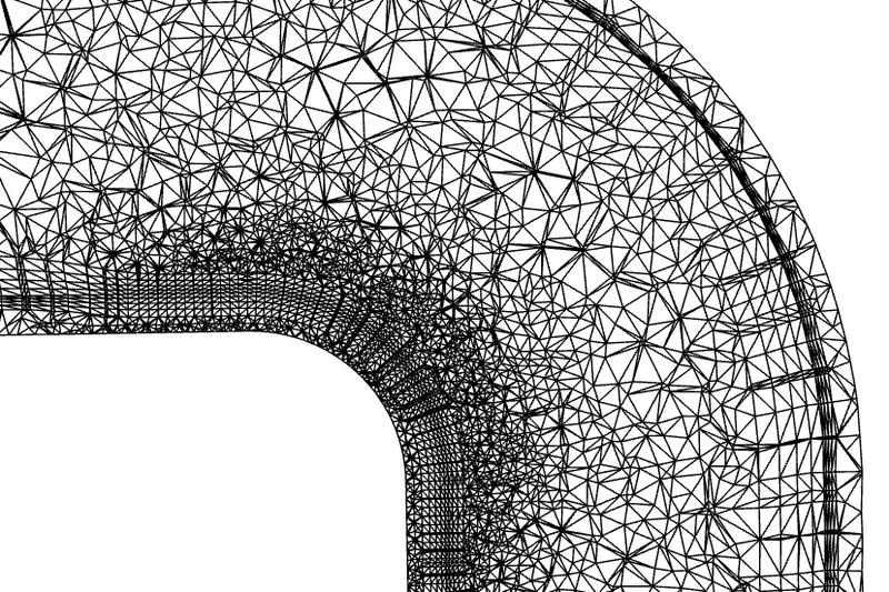
Careful observations of the flow in the baseline mesh were taken to understand regions of flow acceleration to perform the refinement. The refined case was generated with an element sizing of 2.5e-2 m for the solid volume and 1.8e-2 m for the fluid volumes. An edge sizing of 1e-2 m was implemented on the inlets and outlet edges to capture their curvature as done in the baseline. A further refinement using a body of influence was performed at the bend downstream of the intersection of all the inlet pipes near the outlet. This body of influence was made to encompass only the mesh elements at the bend and was given a sizing of 4e-3m. The reduction in the element sizing resulted in the refinement of the inflation layers in the region as well due to the smooth transition mechanism which will aid in the improvement of the wall `y^+`. The resulting refined mesh was generated with 500k cells and can be seen below:
Solver and Boundary Conditions
The analysis was performed on Ansys Fluent 2022 R2. A velocity inlet boundary condition was used at all the inlets with a specified velocity magnitude of 5m/s and temperature of 700K. The pressure outlet boundary condition was applied at the outlet with 0 gauge pressure. The outer wall of the exhaust port was provided with a convective heat transfer coefficient of 20 W/(`m^2`K) and a free stream temperature of 300K. All other walls were made to be adiabatic. The diameter meter of the pipe at the inlet = 0.166m was used as the reference length and a reference temperature of 300K was used for all calculations.
The steady-state pressure-based PV coupled scheme was used for the discretization of the flow parameters. The fluid used in the analysis was air and the solid material was aluminium with their default material properties. The energy equation was enabled for the analysis. The realizable K-Epsilon model with standard wall functions was used to model the turbulence and the near-wall flow. The second order scheme was used to estimate the pressure, the second order upwind scheme was used to estimate momentum and energy and the first order upwind scheme was used to estimate the turbulence parameters. The solution was initialized by hybrid initialization followed by an FMG initialization to quicken the simulation. The simulation was run with pseudo transient time stepping with an automatic global conservative length scale. Convergence was checked by the scaled residuals to reach 1e-3 and the variations in the temperature at the outlet and the area-weighted average of the surface heat transfer coefficient of the pipe not exceeding 1e-3 across iterations.
Analytical estimation of Heat transfer Coefficient
In order to verify the predictions of the heat transfer coefficients from the analysis, analytical estimations can be performed using empirical relations. One such method to compute the heat transfer coefficient is using the Dittus-Boelter equation [1] which estimates the Nusselt number for turbulent flow as:
`Nu_D = 0.023 (Re_D)^(4/5) Pr^0.4`
where,
D- Diameter of the pipe [m]
Re- Reynolds number of the flow [-]
Pr - Prandtl number of the flow [-]
Reynolds number:
`Re = (rho V D )/ mu`
Prandtl number:
`Pr = (C_p mu )/ K`
where,
rho - density of the fluid [kg/`m^3`]
V - free stream velocity [m/s]
D - Characteristic length/ pipe diameter [m]
mu - Dynamic viscosity [kg/m/s]
C_p - Specific heat capacity [J/kg/K]
K - Thermal conductivity [W/m/k]
The Dittus-Boelter equation is valid for:
0.6 `<=` Pr `<=`160
Re `>=` 10,000
L/D `>=` 10
The Nusselt number relates to the heat transfer coefficient by:
`Nu = (hL)/K`
Which can be rewritten as:
`h = (Nu K )/L`
where,
h- Heat transfer coefficient [W/(`m^2`K)]
L - Characteristic length (or pipe diameter in this case) [m]
K - Thermal conductivity [W/m/k]
Upon estimating the Nusselt number from the Dittus-Boelter equation, the heat transfer coefficient can thus be easily estimated from the above relation.
Results
An evaluation of the simulation performance of the initial baseline mesh was conducted to understand the flow field and make refinements in the appropriate regions. The scaled residuals of the two meshes across the iterations simulated are shown below:
Baseline mesh residuals Refined mesh residuals
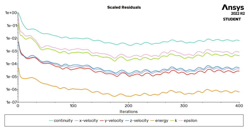
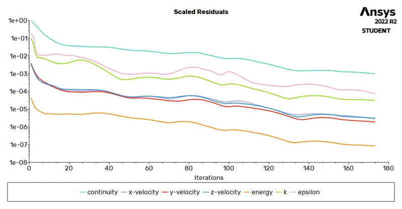
The baseline mesh was not able to bring the scaled residuals below 1e-3 and was generally unstable throughout the iterations. The refined mesh on the other hand has a smoother residual plot and was able to converge well within 180 iterations. This is a clear indication that the mesh refinement worked well and therefore all post-processed results will be shown from the refined mesh case.
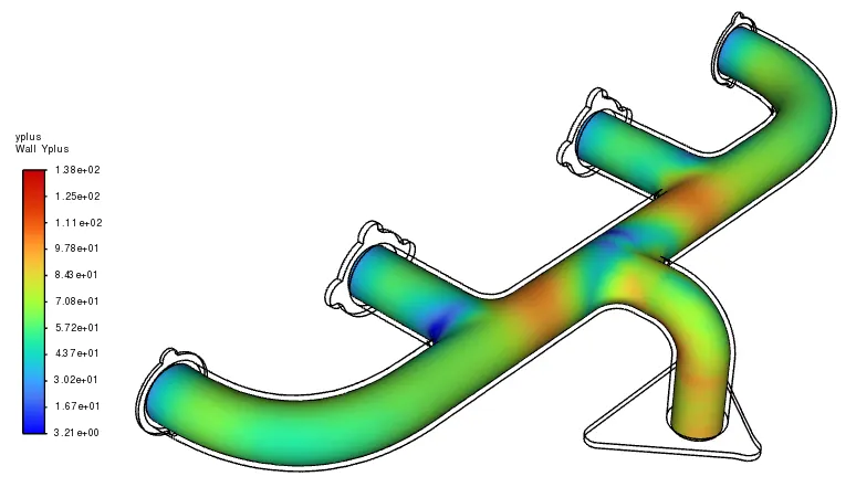
The `y^+` of the refined case on the inner walls of the exhaust port is shown below. The majority of the region is within the 30>`y^+`>100 requirement of the standard wall functions. However, a few regions are still either below a `y^+` of 30 or greater than 100. Ideally, the entire region should be within the 30>`y^+`>100 limit but due to the limitations in the academic license (512k cells), it is not possible to generate such a mesh without compromising the volume mesh transition. A gradual transition of the volume mesh from inflation layers to the bulk mesh is crucial as it affects the predictions of the wall shear stress and wall heat transfer which are both important in a conjugate heat transfer analysis.
The variations in the average heat transfer coefficient and the average outlet temperature across the iterations are shown below:
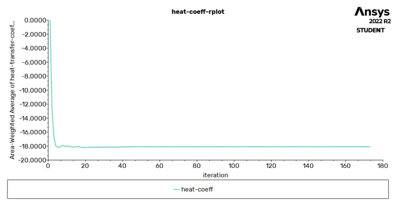
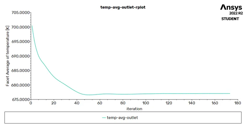
The averaged heat transfer coefficient can be seen to stabilise quickly compared to the averaged temperature at the outlet. Observing these plots along with the scaled residuals makes it clear that the solution has converged. Additionally, from the plot above, the heat transfer coefficient predicted by the simulation is 18.10 W/(`m^2`K).
To visualize the distribution of the surface heat transfer coefficient across the exhaust port, surface contours were generated as seen below:
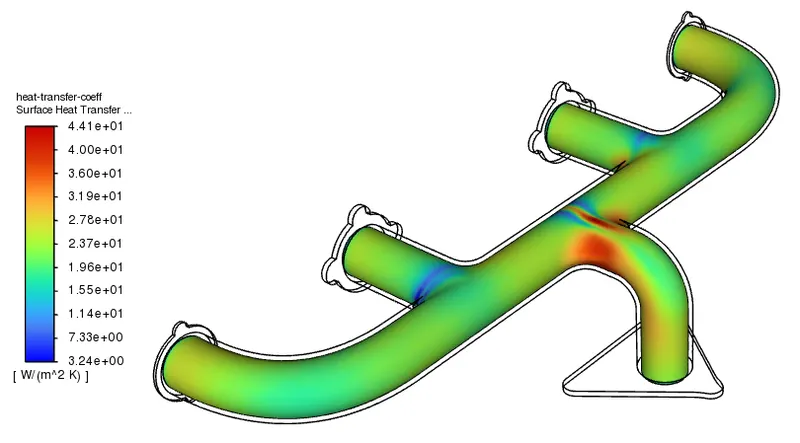
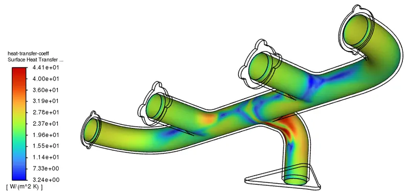
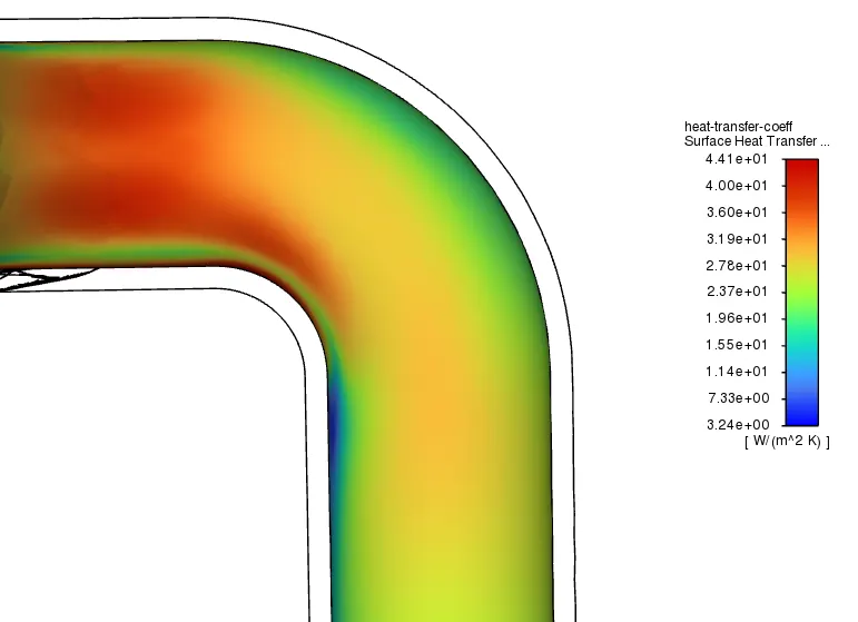
The region with the highest heat transfer coefficient can be seen at the junction where all the inlet channels meet.
The contours of temperature at various planes along the exhaust port and surface of the exhaust port are shown below:
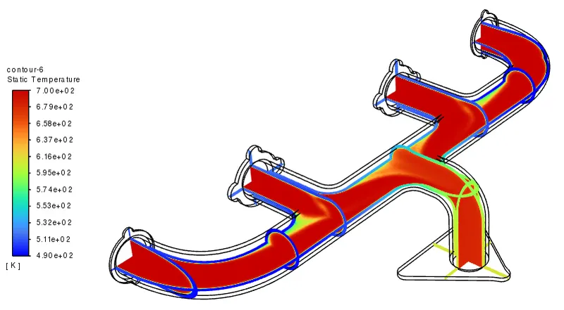
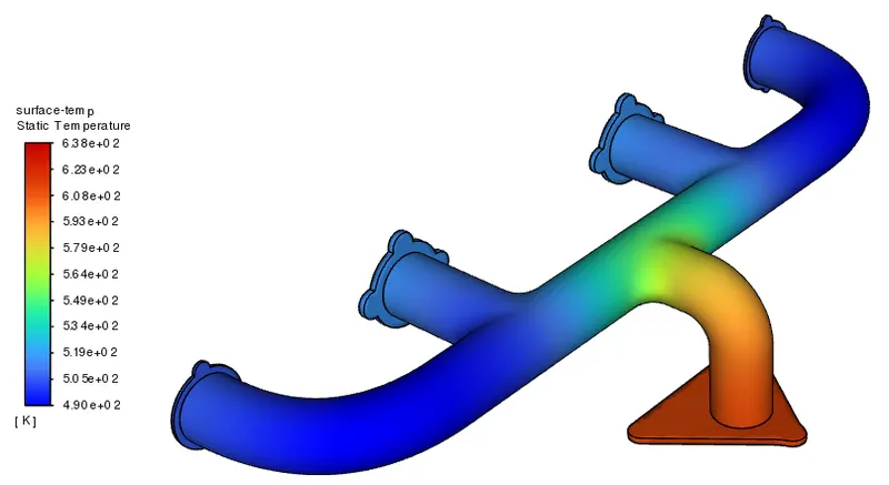
Inside the fluid volume, the temperature at the outlet is lower than the inlet temperature due to the transfer of heat to the solid aluminium. Correspondingly in the solid volume, the temperature at the inlet is lower than the temperature at the outlet as the fluid transfers the heat to the solid. A high temperature on the solid can be seen at the bend where all the inlet channels meet.
The contours of velocity magnitude overlayed with pathlines coloured by velocity are shown below:
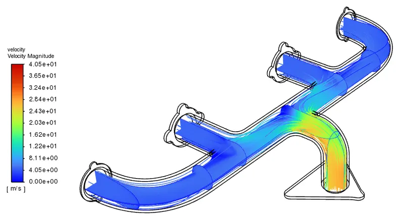
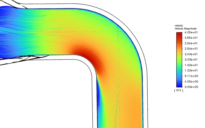
An increase in velocity is observed at the bend near the outlet and is caused due to conservation of flow rate as the entire flow from all inlets is made to pass through this bend. This increase in flow velocity also increased the local wall `y^+` at the area and is the reason behind the local mesh refinement using the body influence in the refined mesh case.
Estimation of Empirical Heat Transfer Coefficient and comparison with the results of simulation
Estimation of flow Reynolds number
Re = 1.225*5*0.166/1.7894e-5
Re = 56820 [-]
Estimation of Prandtl number
Pr = 1006.43* 1.7894e-5 / 0.0242
Pr = 0.744 [-]
Both Reynold's number and the Prandtl number are within the valid region for the application of the Dittus-Boelter equation.
Estimation of Nusselt number using the Dittus-Boelter equation
Nu = 0.023*56820^(4/5) * 0.744^0.4
Nu = 130.01 [-]
Estimation of empirical heat transfer coefficient
h = 130.01* 0.0242 / 0.166
h = 18.95 W/(`m^2`K)
The result from the simulation for the heat transfer coefficient is 18.10 W/(`m^2`K) which constitutes an error of under 5% compared to the empirical results. Hence, the results of the heat transfer coefficient can be deemed validated.
Further increase in accuracy of the simulation prediction can be done by refining the mesh further with finer inflation layers leading to a better wall `y^+`. It should also be noted that in the current analysis, the boundary layer flow is modelled using wall functions. A more accurate prediction of boundary layer flow can be obtained by resolving the boundary layer directly by having mesh elements at `y^+`= 1, which is inside the viscous sublayer of the boundary layer. However, this procedure will increase the mesh size and the computational cost of the simulations.
Higher fidelity CFD models like LES or hybrid LES can also be considered which will increase the overall cost of the simulations but will be able to predict temporal and spatial prediction of parameters with much higher accuracy.
Conclusion
A conjugate heat transfer analysis over the given exhaust port was performed with an inlet flow of air at 5m/s and 700K with aluminium as the material for the solid volume of the exhaust port. An initial baseline mesh was generated followed by a refined mesh based on the results of the baseline case. Contours of velocity, temperature and heat transfer coefficient were plotted to understand the flow inside the exhaust port. Finally, the results of the heat transfer coefficient from the simulation were compared to the empirical solution and observed to differ by under 5%. Due to the small percentage difference, the simulation results for the heat transfer coefficient can thus be deemed validated.
References
- R.H.S. Winterton, Where did the Dittus and Boelter equation come from?, International Journal of Heat and Mass Transfer, Volume 41, Issues 4–5, 1998, Pages 809-810, ISSN 0017-9310, https://doi.org/10.1016/S0017-9310(97)00177-4.