Week 4 - CHT Analysis on Exhaust port
1. Introduction
1.1 Conjugate Heat Transfer (CHT)
Conjugate Heat Transfer (CHT) is the transferring of heat at the interfaces of solids and fluids. The Conjugate Heat Transfer (CHT) analysis type enables the computation of heat exchange across solid and liquid phases for which it is mainly employed in the simulations involving heat exchangers. The simulation of heat transfer, the cooling of electronic devices, and general-purpose cooling and heating systems are examples of typical uses of this analysis type.
1.2 What is y+ Value according to Turbulence Value
The y+ Value is a quasi distance Value. It is frequently utilised to specify the coarseness or fineness of a Mesh Elements for a specific fluid flow pattern. The correct element size at grain boundary must be determined in turbulent simulation. The y+ value at the boundary is constrained by the turbulence model wall laws and the experimental results. Below is one such representation of the y+ Turbulence model.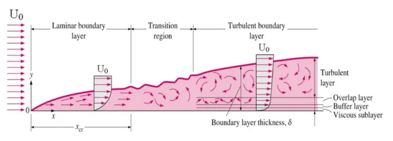
As of general rule:
`y+ = rho * u* y / (mv)`
u* = friction velocity
y = distance from wall
mv = dynamic viscosity
2. Problem Statement
- Give a brief description of why and where a CHT analysis is used.
- Maintain the y+ value according to the turbulence model and justify the results.
- Calculate the wall/surface heat transfer coefficient on the internal solid surface & show the velocity & temperature contours in appropriate areas.
- How would you verify if the HTC predictions from the simulations are right? On what factors does the accuracy of the prediction depend on?
3. Problem Setup for Simulation
3.1 Geometry Setup
- The geometry provided is imported into SpaceClaim for extracting the volume of the geometry as the main aim of the assignment is to understand the flow within this volume.
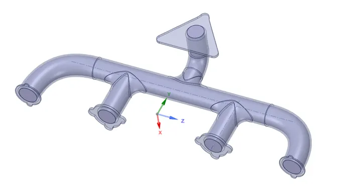
- The Volume is created in another domain along with the existing Solid domain. This needs to be brought together into one domain as represented below.
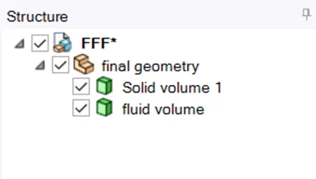
- The topology of the created enclosures needs to be Shared in-order to create the interference between the solid and fluid domains. For this, the Interference tool needs to be utilised and to be made sure that the topologies are shared.

3.2 Mesh Setup
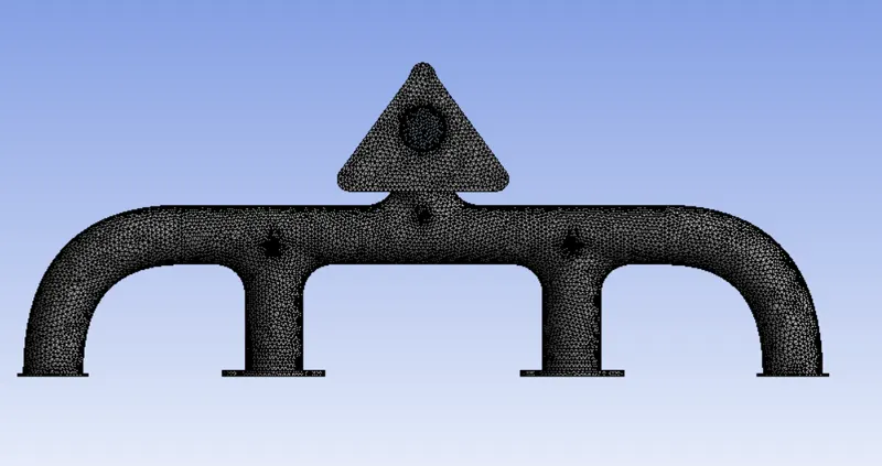
- Initially a coarse mesh can be used for the first case of simulation without the second inner enclosure. For the Second and Third cases where an intermediate and Finer Mesh is required, Sizing methods are utilised where in for the First Enclosure, A MultiZone Mesh is to be setup with an element size of 100mm.
- The inflation layer is created using the y+ values for the First Layer thickness and Total Thickness Calculation
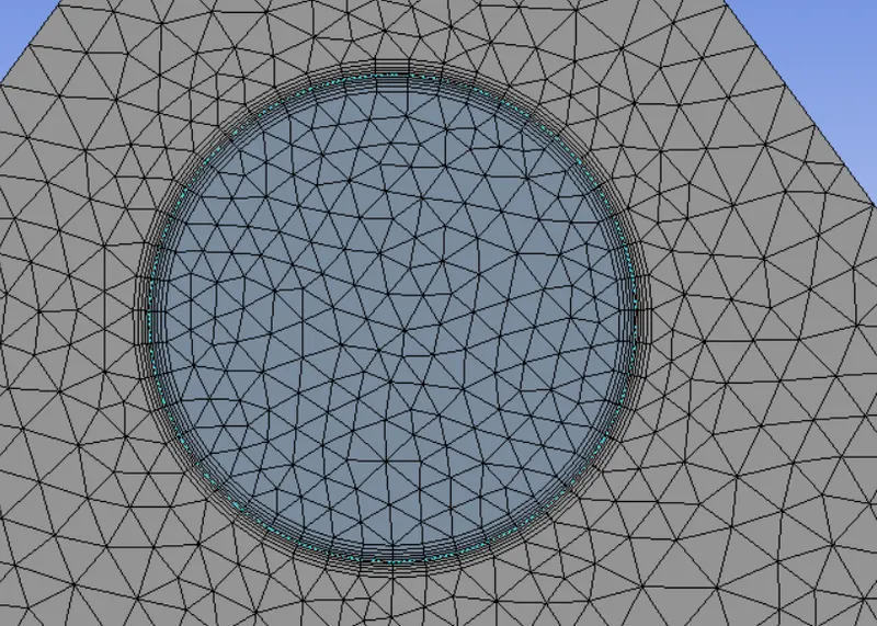
- The final mesh obtined is as represented below.
3.3 Solver Setup
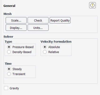
- For Steady State simulation, Steady is selected in the Time Section of the General Tab is to be selected.
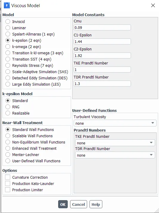
- For all the scenarios, K-Epsilon Flow model is employed.
- The material properties are to be setup as per the requirements, in this case, it is Air and parameters represented are left unchanged.
- A SIMPLE Solution Method is employed.
- The Setup is Initialised and the number of iterations is set to 500 Iterations to obtain the required result.
4. Simulation Results
Case – 1: K-Epsilon
- Velocity Contour and Velocity Streamline of K-Epsilon Model
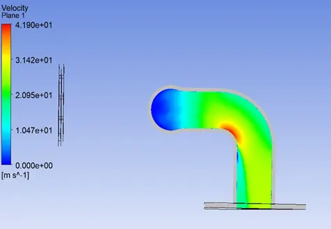
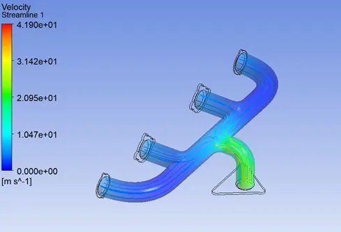
Max: 41.90 m/s; Min: 0 m/s - Temperature Contours of K-Epsilon Model
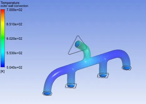
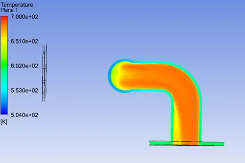
Max: 700 K; Min: 504 K - Heat transfer Coefficients at Inflation layer
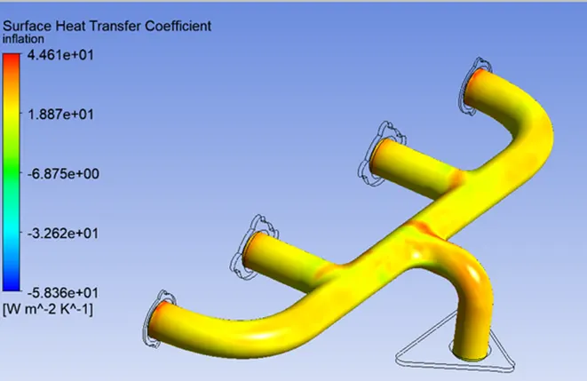
Max: 44.617 W/m2K; Min: -58.36 W/m2K
Case – 2: K-Omega
- Velocity Contour and Velocity Streamline of K-Omega Model
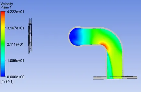
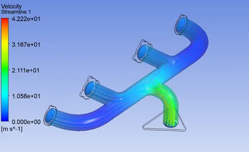
Max: 42.22 m/s; Min: 0 m/s - Temperature Contours of K-Omega Model
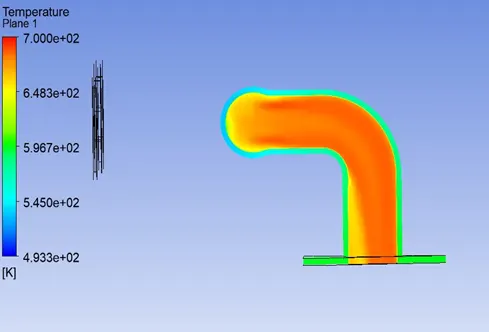
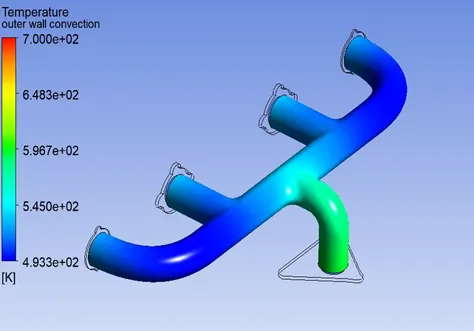
Max: 700 K; Min: 493.3 K - Heat Transfer Coefficients of Inflation Layer
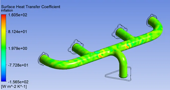
Max: 160.52 W/m2K; Min: -156.5 W/m2K
5. Discussion of Results and Conclusion
Heat Transfer can be determined by using Nusselt Number. The Nusselt number, which measures the convective heat transfer taking place at the surface, is equal towards the non - dimensional temperature difference at the surface. The conductive element is evaluated with a stationary fluid under another circumstances as the heat flux.
`Nu = (h.L)/(Kf)`
Where.
h = Thermal Conductivity of the fluid (W/m.K)
L = Characteristic Length
Kf = Convective Heat Transfer Coefficient (W/m2.K)
As per the above simulation results, it can be observed that the Velocity of the flow is higher near the outlet of the geometry and near the section with a bend for the outlet port. It can be understood from this that the variation in the pressure can cause the change in the velocity and in this case, it can be understood that the pressure at this point is lower.
In the case of the temperatures, it can be observed that the temperature at the outlet seem to increase starting from inlet ports to the outlet ports as the velocity streams mix up to this singular outlet port and also these Velocity Streams tend to increase because of the geometrical aspects like the sudden change in the geometry which can be observed from the above images wherein these turnings in the geometry profile tends to vary pressure and create these high velocity streams.
It can also be understood that the K-Omega is better at solving and capturing Boundary Layer Phenomenon for flow simulation.
6. References
- He, L. and Oldfield, M.L.G., 2011. Unsteady conjugate heat transfer modeling.
- Chen, X. and Han, P., 2000. A note on the solution of conjugate heat transfer problems using SIMPLE-like algorithms. International Journal of Heat and Fluid Flow, 21(4), pp.463-467.
- Shukla, I., Tupkari, S.S., Raman, A.K. and Mullick, A.N., 2012, June. Wall Y+ approach for dealing with turbulent flow through a constant area duct. In AIP Conference Proceedings (Vol. 1440, No. 1, pp. 144-153). American Institute of Physics.