CHT Analysis on Exhaust port

Heat transfer in solids is dominated by conduction and in liquids, it is mostly convection including a negligible amount of heat generation from viscous effects and density dependence on velocity and temperature. Usually, the fluid is the energy/heat carrier. Forced convection is a very common way utilized across various industries for efficient and cheap transfer of heat. But a solid component is required to keep the working fluid separated from the, let’s say, a cooling fluid. The addition of a solid component involves conductive heat transfer, which simply cannot be ignored. That means that the heat transfer methods in such cases are coupled, which in a slightly complex manner is called conjugated.

Conjugate Heat Transfer (CHT) analysis is a type of CFD analysis that allows for the simultaneous stimulation of heat transfer between solid and fluid domains. This is done by exchanging the thermal energy at the interfaces between them.

Why do we have a CHT approach when we have a Finite Element thermal analysis? The answer is simple, the thermal analysis uses simplified empirical equations to solve for heat transfer coefficients, whereas in the CHT approach, these terms and their local variations are directly calculated within the model. Therefore, the CHT approach has an advantage when there is a non-uniform transfer of heat.

CHT approach has applications ranging from analysis of something as small as a chip to something as big as a locomotive railway engine. Such analysis is very important to understand real-time heat transfer and distribution which is essential for the correct functioning of the component while providing the best efficiency. Another case when CHT can be used is when gases alone or trapped in foam, are used as an insulating material, because of their weight and cost advantages.

Rayleigh number

The temperature at which a well patterned “natural convection circulation” is established is called a “critical temperature gradient”.

How to know this critical temperature gradient value?

This is where Rayleigh's number helps us out, it gives you a dimensionless number that easily predicts the critical temperature gradient for establishing a natural convection circulation.

The magnitude of the Rayleigh number is a good indication of whether the natural convection boundary layer is laminar or turbulent.

When the Rayleigh number is small (typically <103), the convection is negligible and most of the heat transfer occurs by conduction in the fluid. For a larger Rayleigh number, heat transfer by convection has to be considered. When buoyancy forces are large compared to viscous forces, the regime is turbulent, otherwise, it is laminar.

Pre-processing

1. Geometry

• Import the geometry into space claim
• Extract the fluid volume using the volume extract option
• Delete the extra edges, if any
• Share topology/share prep, is done to create an interface between the solid and liquid volumes. If this step is missed, then the mesh formed would be an un-conformal mesh.
  
  
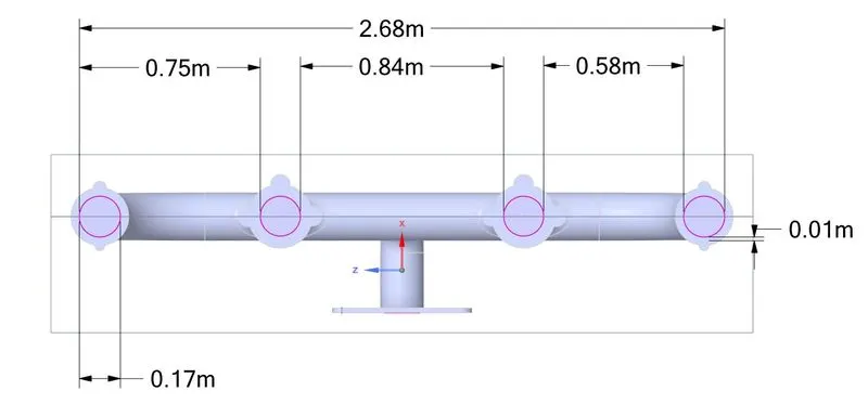
• Inter-face surface area
  
  

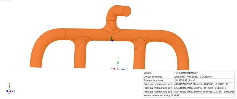
2. Mesh generation

• Give names to the planes, inlets, outlets, etc..
  
  
  
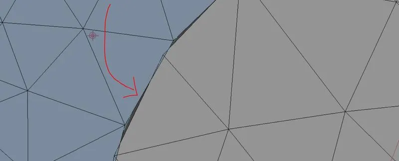
  The above-shown mesh is a proper example of non-conformal mesh, i.e the mesh nodes do not join at the interface, this leads to improper transfer of information at the interface. To avoid this, share topology must be done.
  
  
  
  
  
• Quality of Mesh
  
  
  
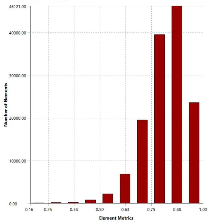
  The Mesh can be further refined to increase the element metrics quality, but this is still a good mesh.

2. Processing/set-up

• Select Energy equation (Since we are dealing with temperature)
• Pressure-based solver (Since M<<0.3)
• Steady-state
• Viscous model - k-epsilon, standard wall function (Almost any model, would give similar results)
• Fluid Material - Air
• Solid Material - Aluminium
• Inlet velocity = 5m/s
• Inlet fluid temperature = 700k
• Outer wall convection rate = 20W/m^2k

3. Results/ post-processing

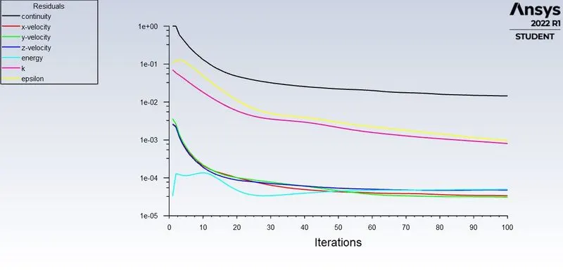
Convergence check

Contours

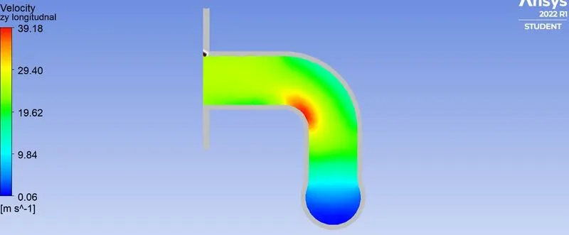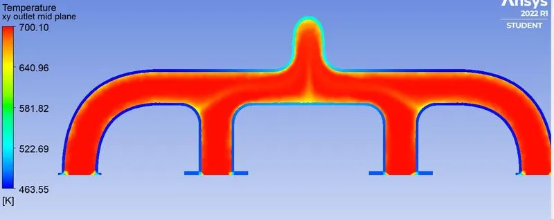
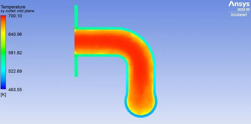
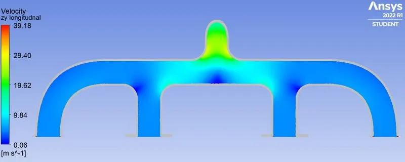
The temperature and velocity plots look correct and makes sense in the fluid region. It can be noticed that the flow velocity almost becomes 7 times the inlet velocity at the outlet bend location. This is to conserve mass flow rate.

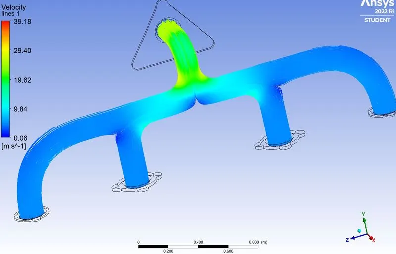
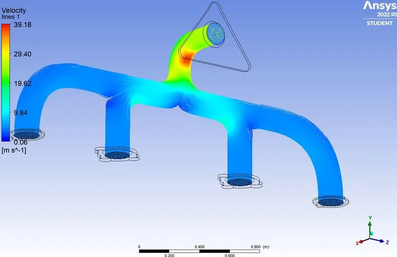
This can be properly observed in using streamlines as shown below.

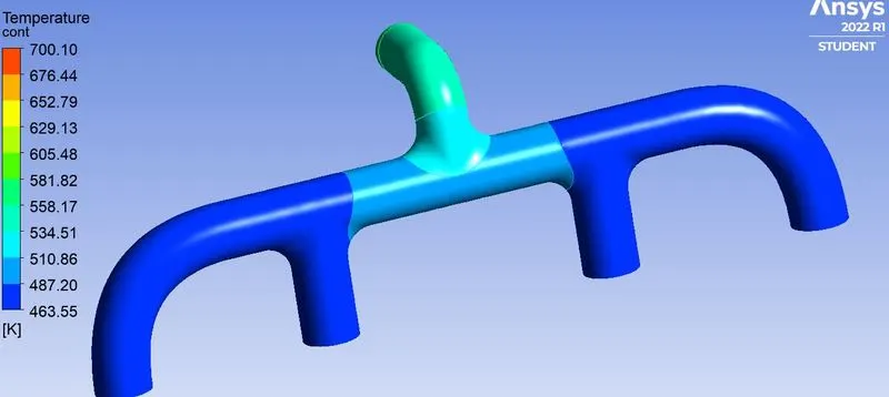
Outer wall temperature increases at the outlet bend as shown below.

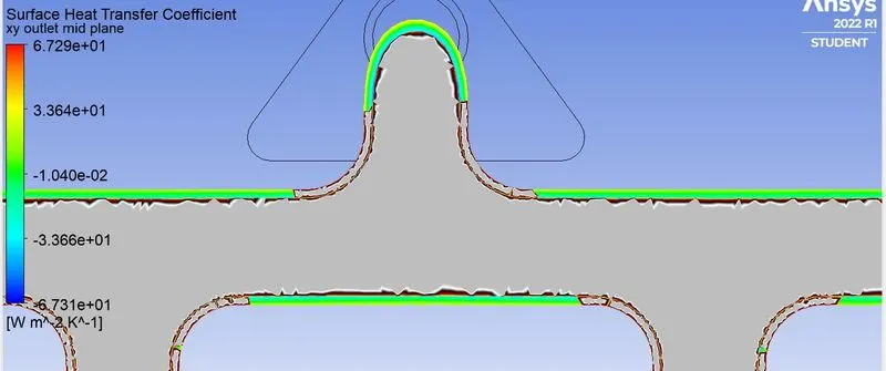
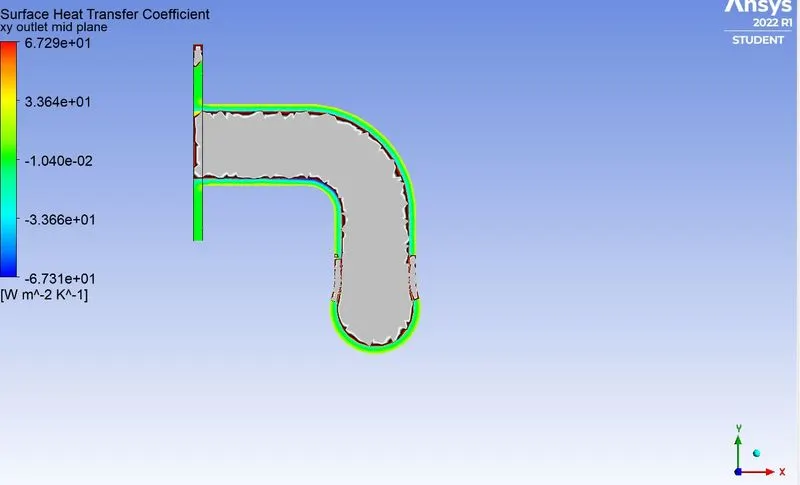
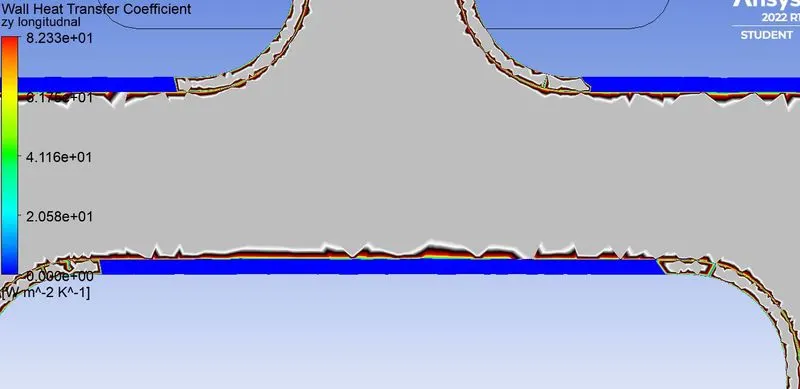
Surface and heat transfer coeff plots

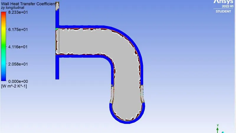The above contours do show some colors/data but don't make much sense. To know if these contours are actually correct or not, we must look at the quantitative plots and y+ data.

• Surface heat transfer plot
  
  
  
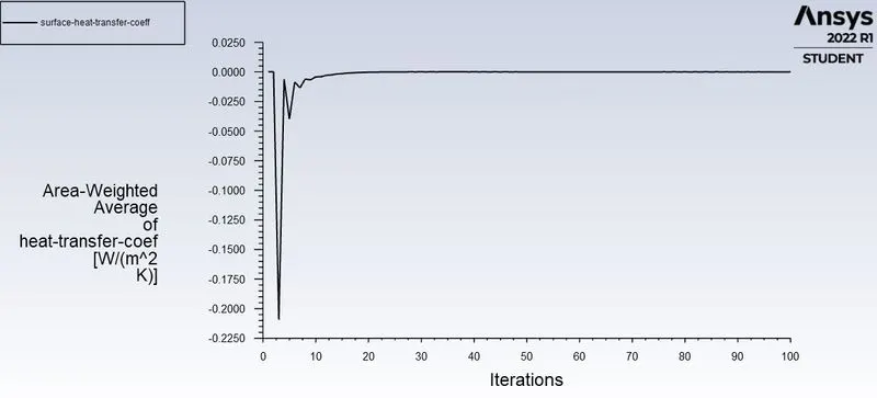
  This plot definitely doesn't make sense, the average heat transfer coeff cannot be zero unless it is an adiabatic structure.
  
  
• y-plus plot
  
  
  
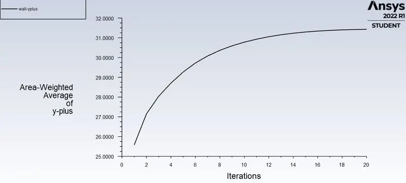
  The high value of y-plus of our mesh explains why our results do not make much sense. The Mesh must be further refined for meaningful results.

Re-Meshing/Refinement

A y-plus of 1 or lower than 1 perfectly captures the effects near the boundaries.

Appropriate first layer thickness calculation for a y-plus of 1

`Re=(rhovd)/mu`

Using the above formula, the Reynolds number at the inlet can be found as 58189.896. This clearly shows that the fluid flow is turbulent in nature.

The coefficient of friction for internal flows which are turbulent in nature is given by,

`C_f=0.079Re^-0.25`

`C_f=0.005086`

The wall shear stress is given by,

`tau_w=0.5rhov^2C_f`

`tau_w=0.077879`

The velocity plus is given by,

`u_tau=(tau_w/rho)^0.5`

`u_tau=0.2514`

The first layer thickness is calculated using,

`Deltay_1=(mu)/(rhou_tau)`

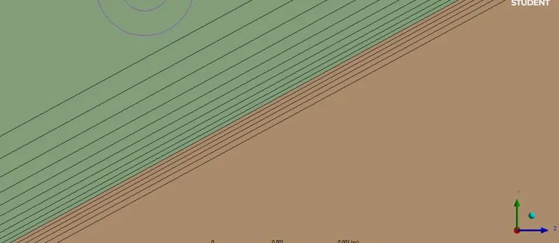
`Deltay_1=0.057933 mm`

Adding inflation layers at the solid-liquid interface as per above calculation.

Results

• y-plus plot
  
  
  
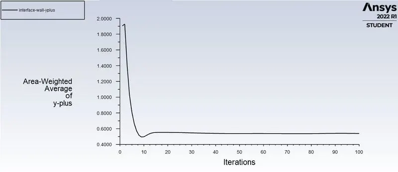
  A y-plus of less than 1 or close to 1 captures the interface/wall physics perfectly.
  
  
  
• Residuals
  
  
  
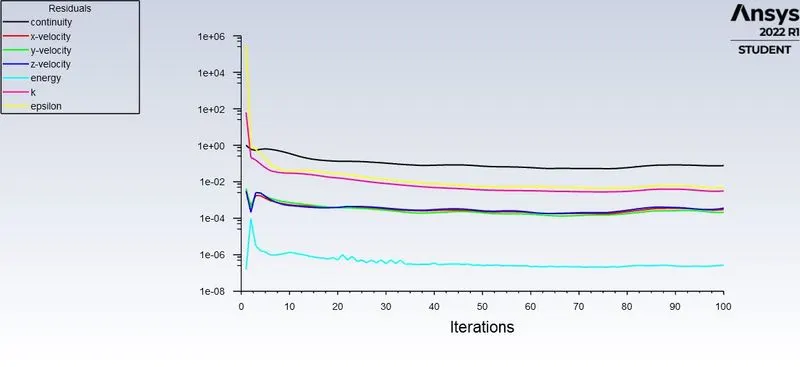
  The residuals show that the simulation has converged at around 50 iterations.
  
  
  
• Surface heat transfer coefficient plot
  
  
  
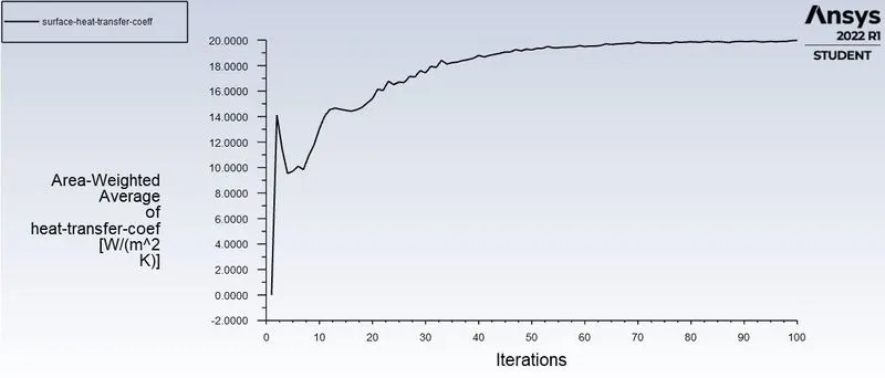
  A surface heat transfer coefficient around 20W/m^2k makes perfect sense, as it is equal to the convective heat flux rate prescribed during set-up.
  
  
  
• Wall heat transfer coefficient
  
  
  
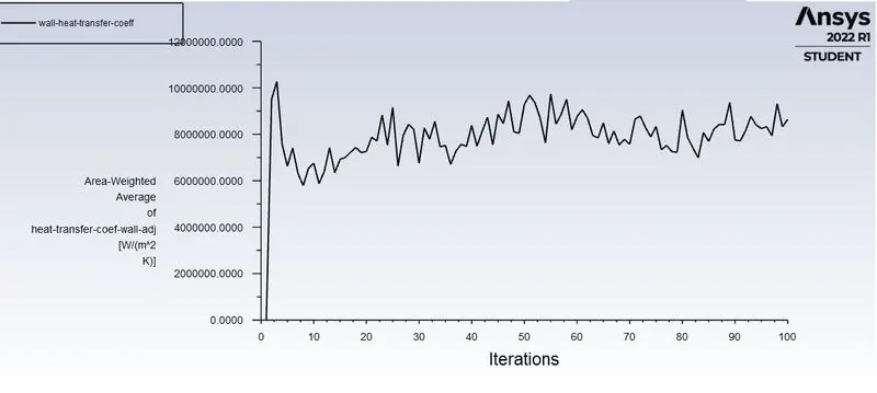
  The above results may look very absurd and incorrect, but they are more or less correct. These can be validated analytically using the formula,
  
  `Q=h(DeltaT)A`
  
  Where,
  Q is the total heat flux
  `DeltaT`is the difference in bulk temperature and reference temperature
  and A is the total surface area.
  
  For, further understanding of the wall heat transfer coefficient and its calculation. Please read the Ansys user manual.
  
  
• Total Heat Flux
  
  

Validation

Prandtl number, `Pr=muC_p/k`

pr number of air = 0.74 ( can be calculated using above mentioned formula, or is available in standard graphs for properties of air.

Nusselt's number, `Nu=0.023Re^0.8Pr^0.3`

Nusselt's number at Re = 58189.896 is 136.2609

Heat transfer coefficient, `h=k/dNu`

Heat transfer coefficient = 19.2368.

Thus, the heat transfer coefficients obtained from the analytical solution and numerical solution match closely and the error percentage is minute.