Week 4 - CHT Analysis on Exhaust port

AIM:

We are to simulate a Conjugate Heat Transfer (CHT) on an exhaust port model with 4 outlets and 1 inlet and find answers to the following series of questions:

• Why and where a CHT analysis is used?
• Maintain the y+ value according to the turbulence model and justify the results.
• Calculate the wall/surface heat transfer coefficient on the internal solid surface & show the velocity & temperature contours in appropriate areas.
• How would you verify if the HTC predictions from the simulations are right? On what factors does the accuracy of the prediction depend?

INTRODUCTION:

Heat Transfer generally takes place through three modes - Conduction, Convection and Radiation. CHT analysis is carried on when we are trying to understand the heat transfer between fluids and solids. This type of simulation involves both conduction(solids) and convection(fluids) and further forced and natural convection as well.

CHT applications include any case where fluids and solids share boundaries and where both heat transfer characteristics are important to evaluate the case. Some examples include Cooling Fins, Electronic Cooling, Heat Exchangers and the list goes on.

GEOMETRY:

We have an exhaust port model, We will prepare the model by using the volume extract tool and then enable the share topology method so that the fluid and solid bodies form a unified conformal mesh at the point of their contact.

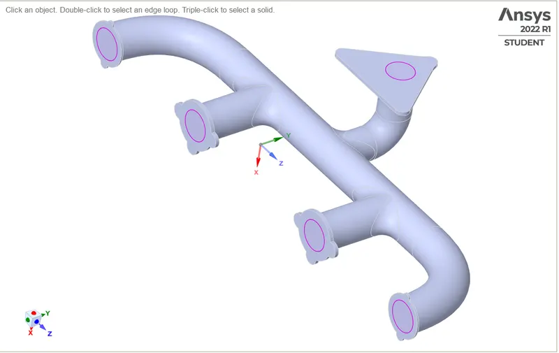
Geometry after enabling shared topology

MESHING:

To refine the mesh, we will follow two methods:

• Refine the solid mesh by increasing the number of elements
• Add inflation layer to the fluid volume using wall functions

The outer solid body element size has been reduced to 15mm for a finer mesh: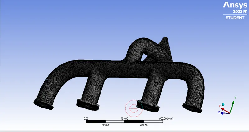

and the fluid volume has been supplied with an inflation layer to capture the wall effects:

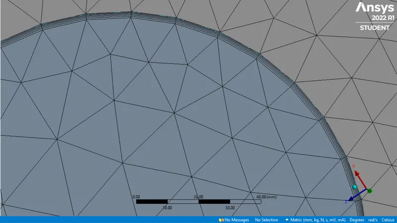
using yplus according to our parameters:

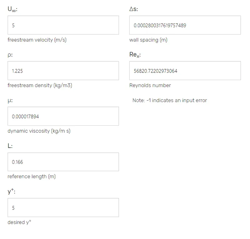
SOURCE: https://www.cadence.com/ko_KR/home/tools/system-analysis/computational-fluid-dynamics/y-plus.html

For Komega model y+<=10

RESULTS:

TEMPERATURE PROFILE:

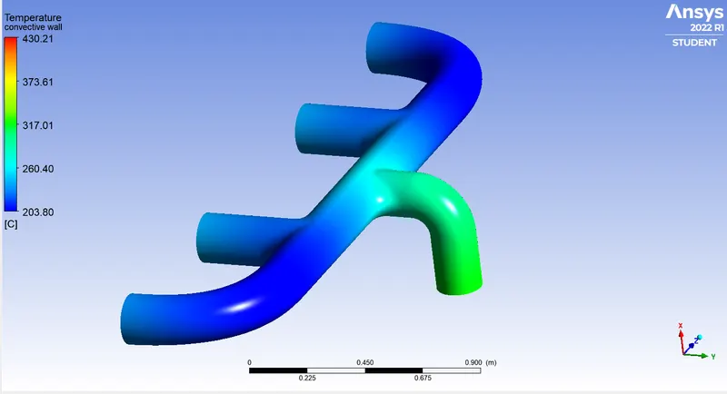
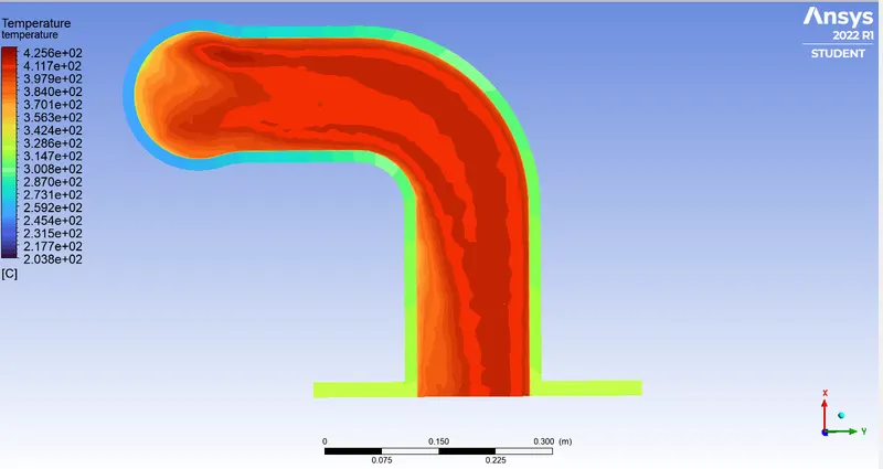
VELOCITY PROFILE:

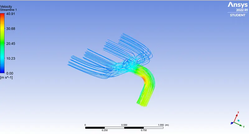
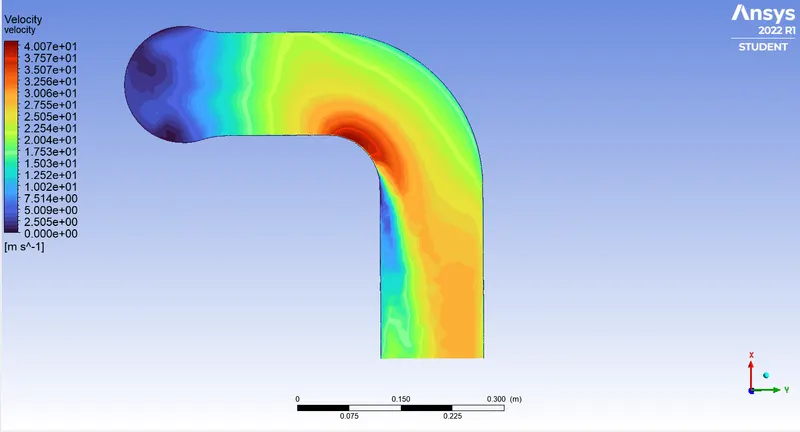
HTC: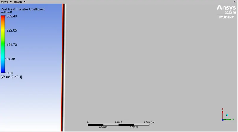

VERIFICATION:

`Re_D` = 56820.7

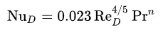
From Dittus-Boelter Equation:

Prandtl Number:

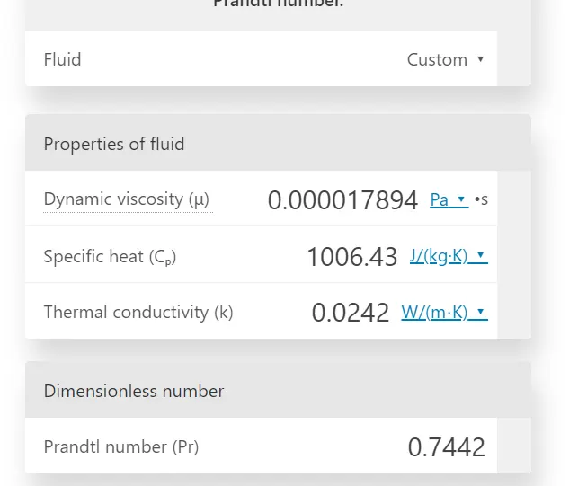
Source:https://www.omnicalculator.com/physics/prandtl-number#example-using-the-prandtl-number-calculator

Substituting the values in Dittus-Boelter, we get Nu = 130

We know that:

substituting, we get h = 18.95 `W/m^2K`.

FACTORS AFFECTING ACCURACY:

There are some general parameters which affect the accuracy:

• Mesh Size: A refined mesh gives a more accurate result, however, it's a tradeoff between performance and accuracy
• Wall Function: Wall functions help enhance wall treatment and give more accurate results for near-wall flow

Besides these factors, there are other factors, such as the Nusselt number we calculated is a simple calculation in which flow rates, number of inlets and outlets don't play any role. However, in the Simulation result shown above the HTC is local HTC and not average, hence the difference.

Another important factor is choosing the right turbulence model to better simulate the flow and capture turbulence.