Week 4 - CHT Analysis on Exhaust port
AIM:- To Simulate for Conjugate Heat Transfer Analysis on Exhaust port using Ansys FLuent
Objective:-
- Give a brief description of why and where a CHT analysis is used.
Maintain the y+ value according to the turbulence model and justify the results.
- Calculate the wall/surface heat transfer coefficient on the internal solid surface & show the velocity & temperature contours in appropriate areas.
- How would you verify if the HTC predictions from the simulations are right? On what factors does the accuracy of the prediction depend?
Theory:-
Conjugate Heat Transfer (CHT) -
- The Conjugate Heat Transfer (CHT) analysis type allows for the simulation of heat transfer between fluid and solid domains by exchanging thermal energy at the interfaces between them.
- In solids conduction is responsible for heat exchange whereas in fluids convection accounts for heat transfer.
- The principle of conduction is governed by Fourier's law of heat conduction, whereas convection is influenced by Newton's law of cooling.
- In engineering applications, heat transfer problems are complex to solve because of different modes of heat transfer and therefore it needs a numerical model which can approximate the physical process.
- CHT analysis is beneficial in accurately predicting solid temperature and heat transfer capabilities in engineering devices.
Applications of CHT
Heat exchangers - A heat exchanger is a system used to transfer heat between two or more fluids. Heat exchangers are used in both cooling and heating processes. The fluids may be separated by a solid wall to prevent mixing or they may be in direct contact.
Automobile sector - In an internal combustion engine in which a circulating fluid known as engine coolant flows through radiator coils and air flows past the coils, which cools the coolant and heats the incoming air.
Aviation - In commercial aircraft heat exchangers are used to take heat from the engine's oil system to heat cold fuel. This improves fuel efficiency, as well as reduces the possibility of water entrapped in the fuel freezing in components.
CHT analyses are also used in the nuclear domain to calculate the heat transfer rate while cooling nuclear tubes as they generate an enormous amount of heat energy.
CHT analysis can accurately predict heat transfer by simultaneously solving all the relevant solid and flow field heat transfer
Other applications are HVAC (Heating Ventilation and Air Conditioning), Air-cooled and liquid-cooled engines, turbochargers, cooling of nuclear reactors, cooling towers, and many more.
Conjugate heat transfer Analysis on Exhaust Port
Cases
| Cases | Y+ | `Y_H` | Turbulence Model | Mesh Type |
| Case 1 | Baseline | NA | K-epsilon | Coarse |
| Case 2 | 30 | 3.3 | K-epsilon | Refined |
| Case 3 | 5 | 0.56 | K-omega-SST | Fine |
Procedure-
ANSYS Workbench (Fluent) is used for the solution.
Geometry
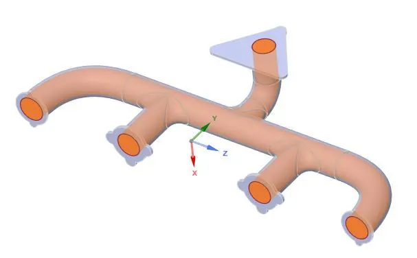
- Import the Exhaust Port model fine in SpaceClaim for cleanup.
- Fluid volume(wet volume) is extracted from the domain as a new component and select share topology to do a multi-body part in Ansys.
- In properties share topology is selected because fluid and solid volumes will be interacting with each other and must share information (heat exchange information) at the interface as a part of the problem.
Meshing:
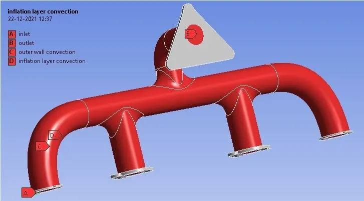
- Assigned names for Inlet, Outlet, walls
CASE - 1
| Mesh Type | Coarse |
| Element Size | 100 |
| `Y_H` (1st cell height) | NA (Baseline) |
| Total number of cells | 136683 |
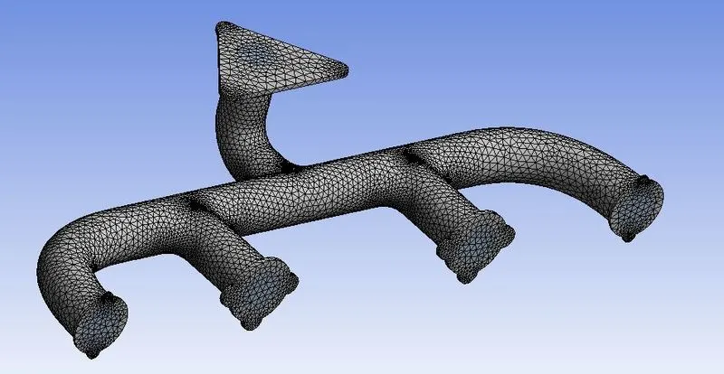
Mesh- A baseline Coarse mesh is created
Setup-
|
Solver Type |
Pressure-Based |
|
Velocity Formulation |
Absolute |
|
Time |
Steady |
|
Viscous Model |
K-epsilon (Standard) |
|
Material |
Fluid type: Air Solid-type: Aluminium |
|
Cell zones |
Fluid type: Air Solid-type: Aluminium |
|
Boundaries |
Inlet Velocity Magnitude - 5m/s Temperature – 700K Outlet - (Pressure outlet) Outer-wall-convection -Wall All other walls - adiabatic |
|
Reference values |
Area = 0.02167m2m2 Length = 0.1661m Density = 1.225kg/m3m3 Enthalpy = 0 J/kg Pressure = 0 pa Temperature = 687.47 K Velocity = 5m/s Viscosity = 1.7894e-05 kg/ms |
Post-Processing Results:
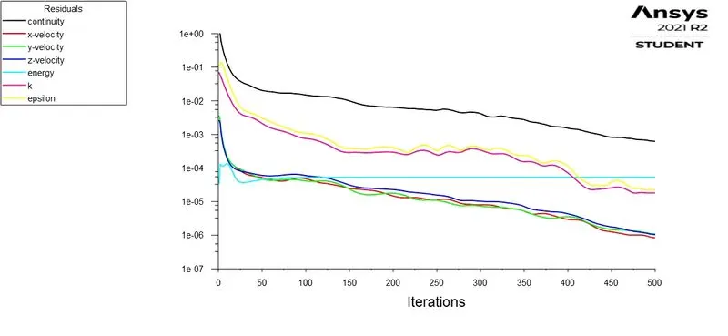
Residuals-
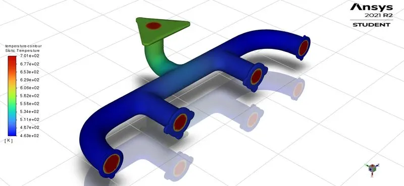
Temperature- Temperature contour graph on Exhaust Port
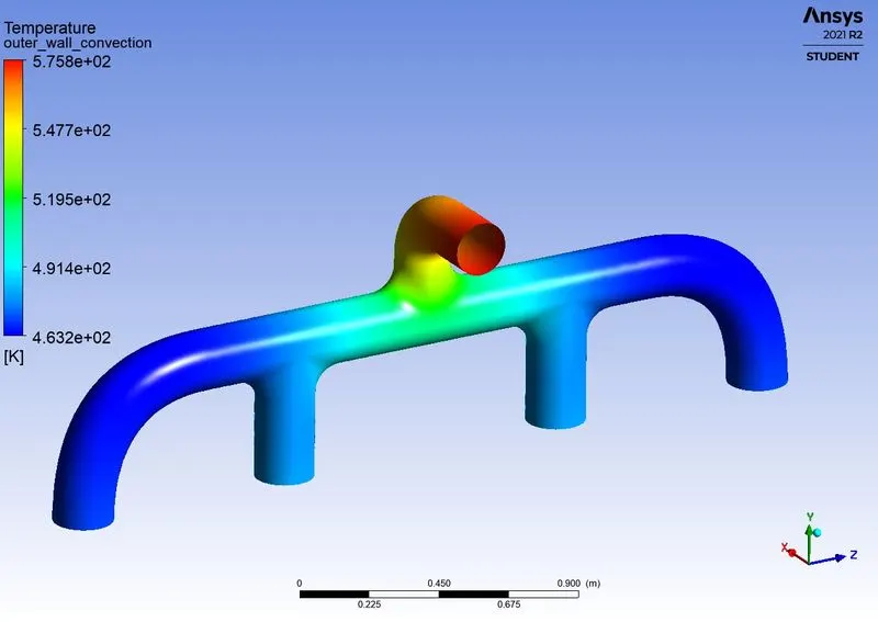
Temperature- Temperature contour graph on Outer Wall
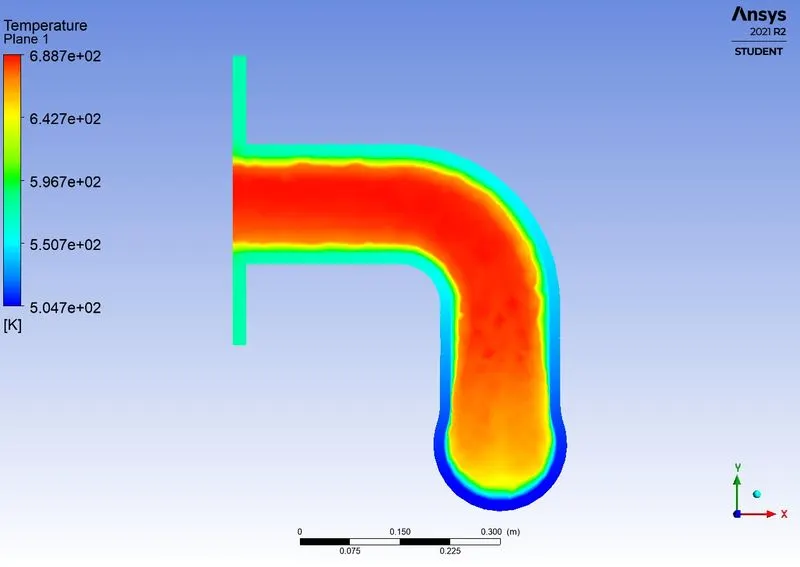
Temperature- Temperature contour graph on a plane
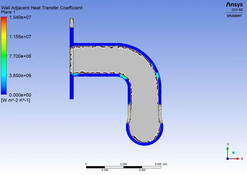
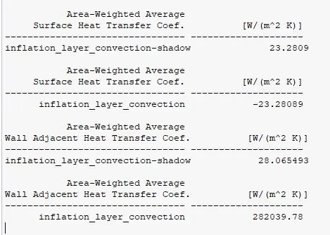
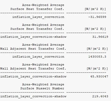
Wall Adjacent Heat Transfer Coefficient
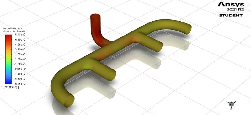
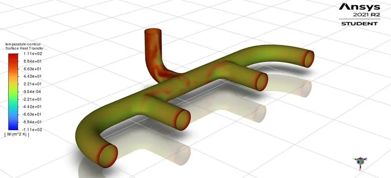
Surface Heat Transfer Coefficient
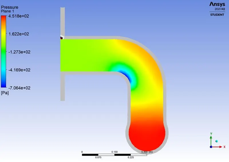
Pressure Contour Plot
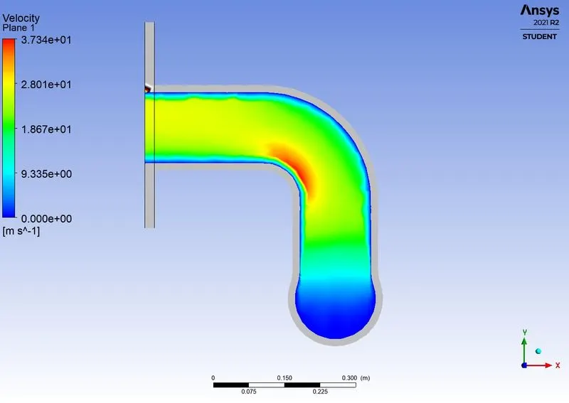
Velocity Contour Plot
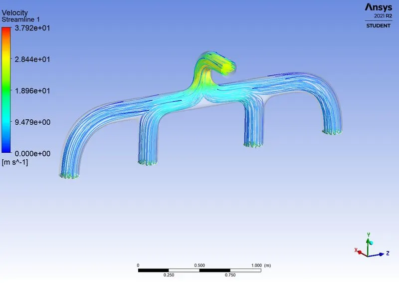
Velocity Streamlines plot- Velocity of Fluids
Reports -
CASE - 2
| Mesh Type | Refined |
| Element Size | 30 |
| Y+ | 30 |
| `Y_H` (1st cell height) | 3.3mm |
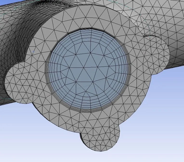
| Number of Inflation layer | 5 |
| Growth Ratio | 1.2 |
| Total number of cells | 209716 |
Mesh- A coarse mesh with an Inflation layer is created.
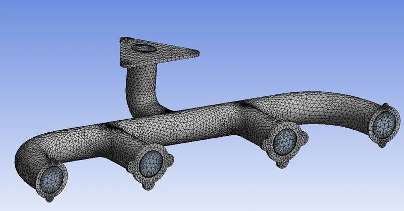
Enlarged View
Setup-
|
Solver Type |
Pressure-Based |
|
Velocity Formulation |
Absolute |
|
Time |
Steady |
|
Viscous Model |
K-epsilon (Standard) |
|
Material |
Fluid type: Air Solid-type: Aluminium |
|
Cell zones |
Fluid type: Air Solid-type: Aluminium |
|
Boundaries |
Inlet Velocity Magnitude - 5m/s Temperature – 700K Outlet - (Pressure outlet) Outer-wall-convection -Wall All other walls - adiabatic |
|
Reference values |
Area = 0.02167m2m2 Length = 0.1661m Density = 1.225kg/m3m3 Enthalpy = 0 J/kg Pressure = 0 pa Temperature = 687.47 K Velocity = 5m/s Viscosity = 1.7894e-05 kg/ms |
Post-Processing Results:
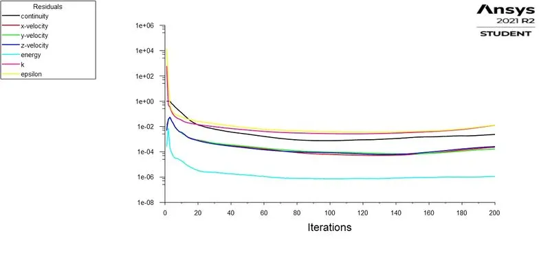
Residuals-
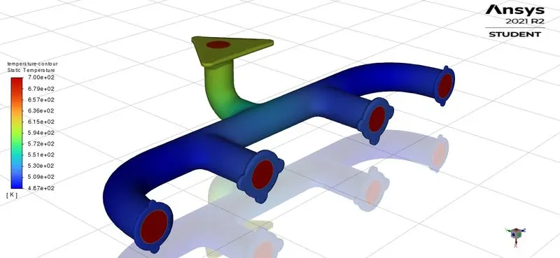
Temperature- Temperature contour graph on Exhaust Port
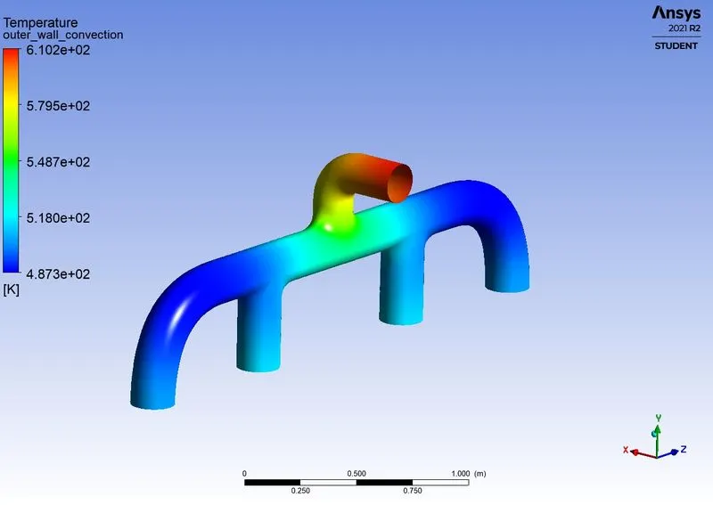
Temperature- Temperature contour graph on Outer Wall
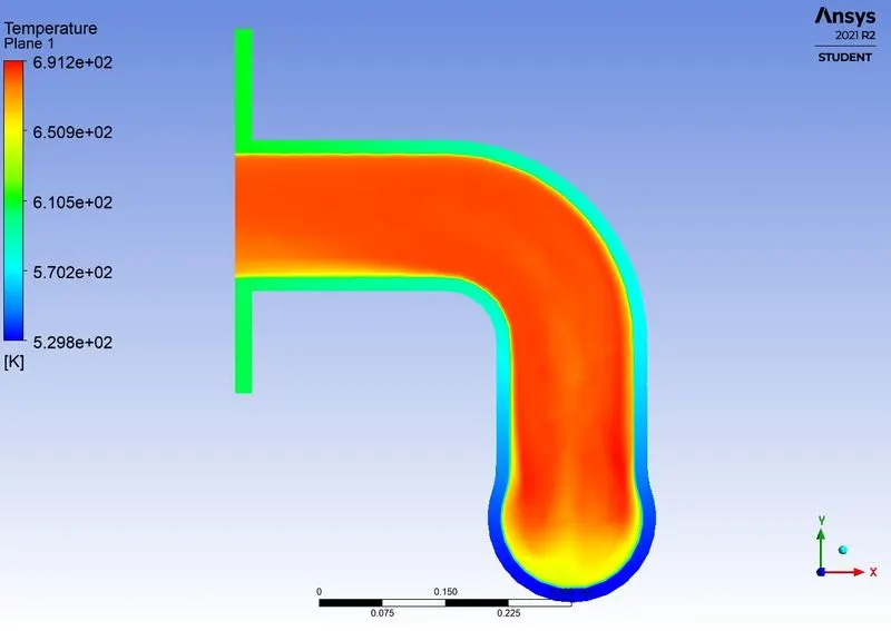
Temperature- Temperature contour graph on a plane
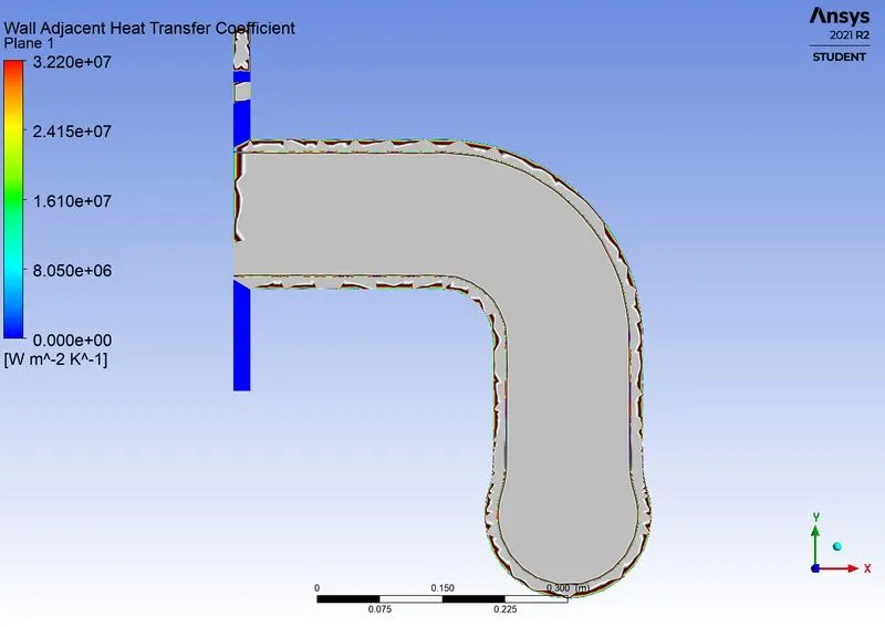
Wall Adjacent Heat Transfer Coefficient
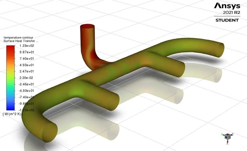
Surface Heat Transfer Coefficient
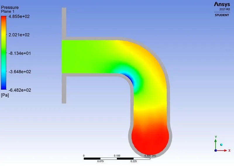
Pressure Contour Plot
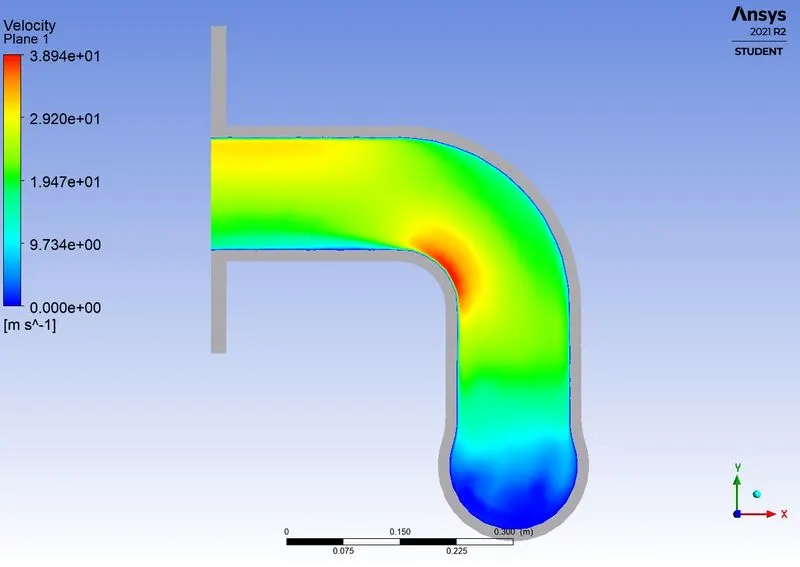
Velocity Contour Plot
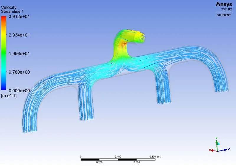
Velocity Streamlines plot- Velocity of Fluids
Report -
CASE - 3
| Mesh Type | Fine |
| Element Size | 15 |
| Y+ | 5 |
| `Y_H` (1st cell height) | 0.56 mm |
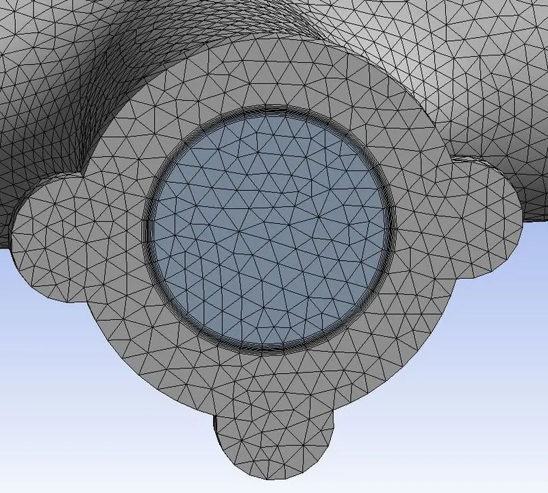
| Number of Inflation layer | 5 |
| Growth Ratio | 1.2 |
| Total number of cells | 483474 |
Mesh- A coarse mesh with an Inflation layer is created.
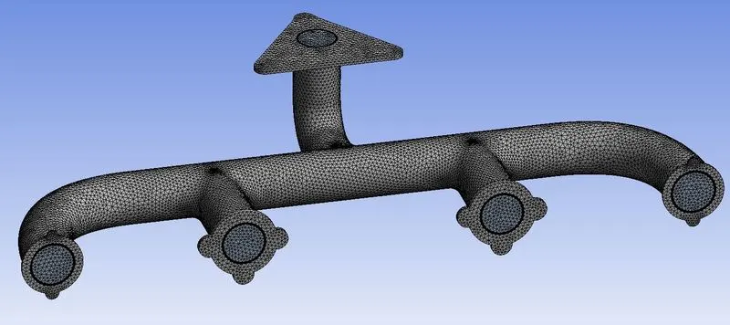
Enlarged View
Setup-
|
Solver Type |
Pressure-Based |
|
Velocity Formulation |
Absolute |
|
Time |
Steady |
|
Viscous Model |
K-Omega-SST |
|
Material |
Fluid type: Air Solid-type: Aluminium |
|
Cell zones |
Fluid type: Air Solid-type: Aluminium |
|
Boundaries |
Inlet Velocity Magnitude - 5m/s Temperature – 700K Outlet - (Pressure outlet) Outer-wall-convection -Wall All other walls - adiabatic |
|
Reference values |
Area = 0.02167m2m2 Length = 0.1661m Density = 1.225kg/m3m3 Enthalpy = 0 J/kg Pressure = 0 pa Temperature = 687.47 K Velocity = 5m/s Viscosity = 1.7894e-05 kg/ms |
Post-Processing Results:
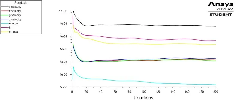
Residuals-
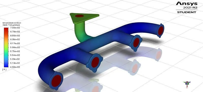
Temperature- Temperature contour graph on Exhaust Port
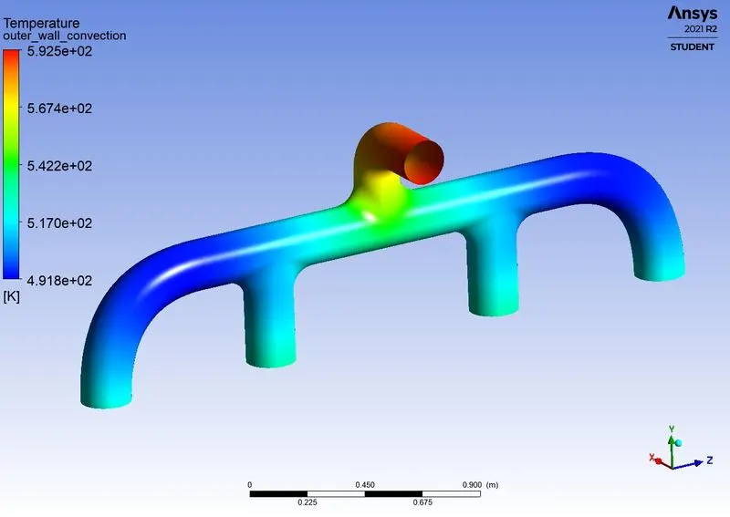
Temperature- Temperature contour graph on Outer Wall
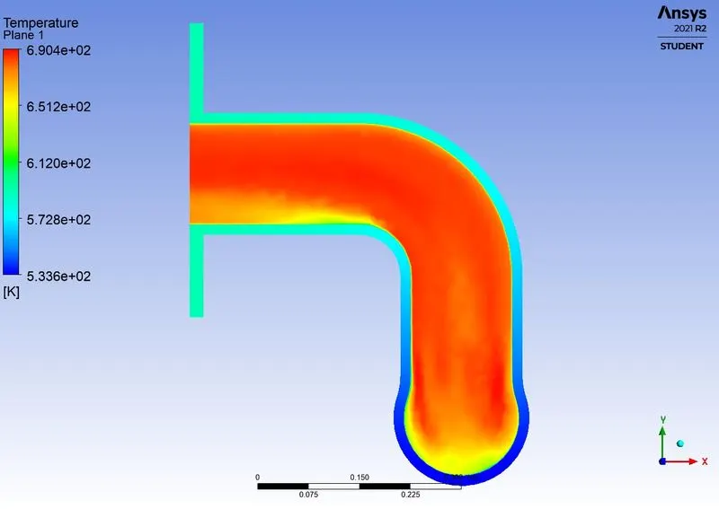
Temperature- Temperature contour graph on a plane
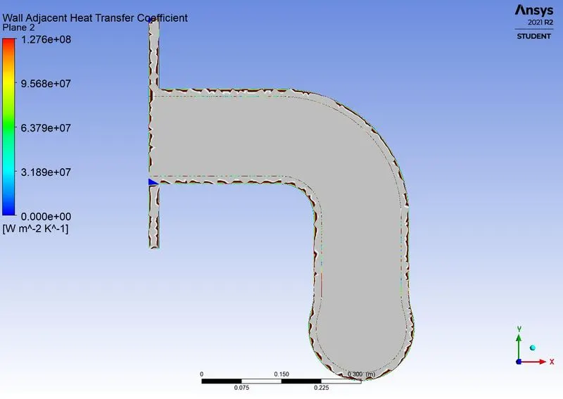
Wall Adjacent Heat Transfer Coefficient
Surface Heat Transfer Coefficient
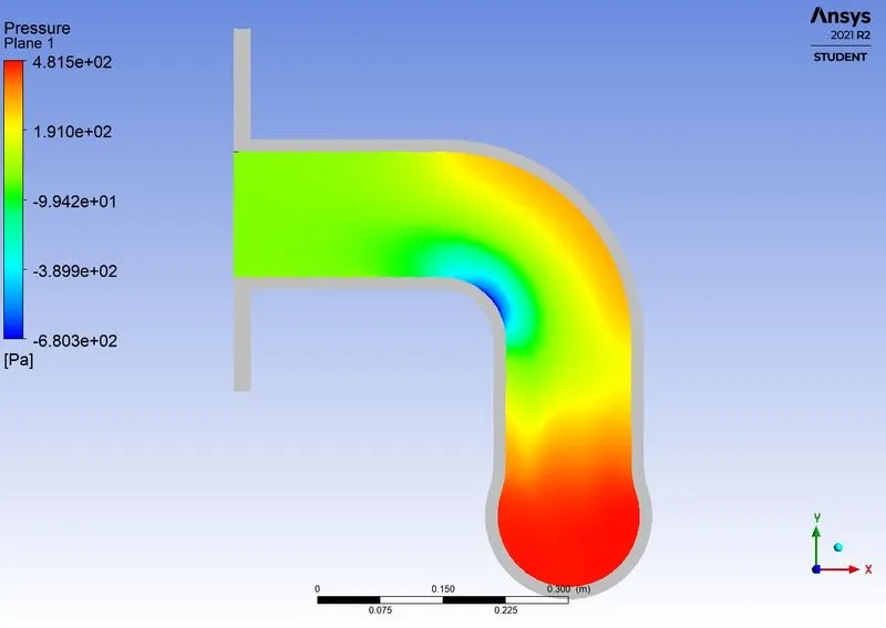
Pressure Contour Plot
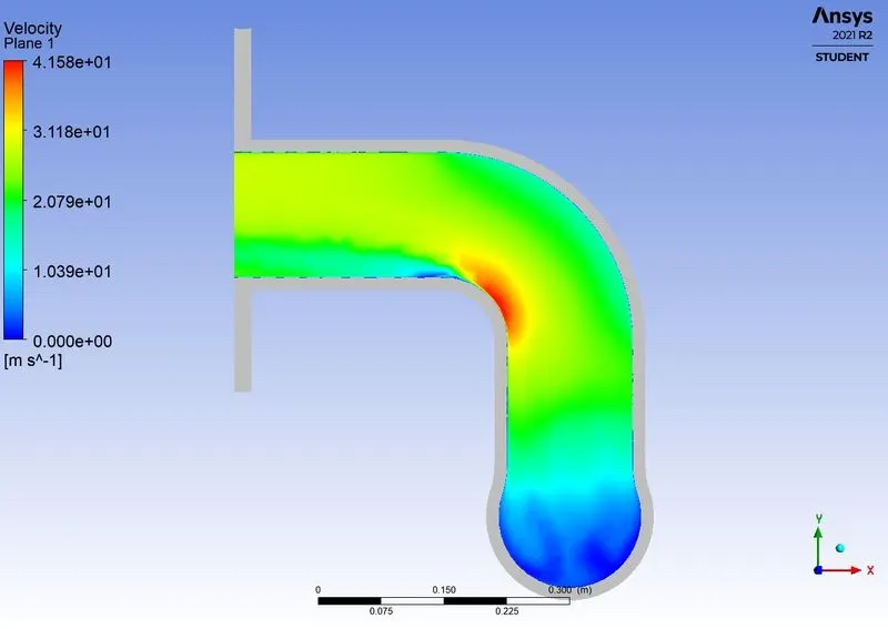
Velocity Contour Plot
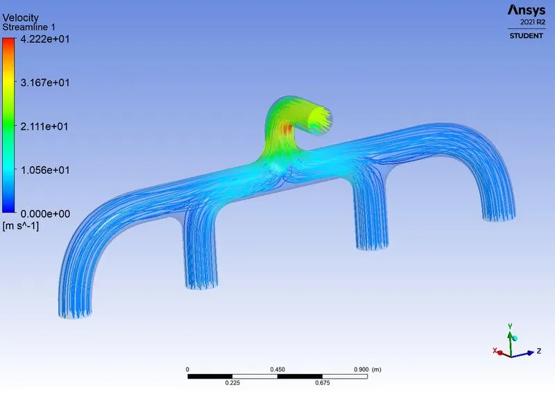
Velocity Streamlines plot- Velocity of Fluids
Report -
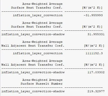
Note-
- Wall adjacent heat transfer coefficient uses the difference of wall temperature and cell temperature adjacent to the wall.
Wall adjacent heat transfer coefficient = wall heat flux/ (wall temperature - wall adjacent temperature)
- Surface heat transfer coefficient uses the difference of wall temperature and reference fluid temperature (bulk fluid temperature).
Surface heat transfer coefficient = wall heat flux / (wall temperature - bulk fluid temperature)
Observation from the cases
- In this problem, the conjugate heat transfer is in between the solid volume of the exhaust port and the heated fluid volume which is flowing through the manifold.
- The heated fluid (exhaust gases) is exchanging heat with the exhaust manifold via convection and the heat by the exhaust manifold is distributed throughout the thickness of the manifold via conduction.
- As a function of fluid flow through the manifold (spatial function), fluid loses its thermal energy and transfers it to internal manifold walls. The rate of heat transfer due to convection is dependent on the velocity of the exhaust gases.
- It can be observed from the temperature and velocity contour. The manifold wall attains maximum temperature where the velocity of the fluid flow is highest, this is due to the high Reynolds number intense turbulence ensures efficient heat transfer.
- The velocity of the fluid is maximum at the bent section of the outlet region. This is because of the continuity (mass conservation) principle, which the domain exhibits. Through four inlets the mass of fluid is entering into the manifold and it has a single way out at the outlet section.
- The maximum velocity region contributes to the maximum heat transfer coefficient. As discussed earlier, the rate of heat transfer is a function of the velocity of the fluid. Heat flux in this region is maximum and results in a high heat transfer coefficient. Accordingly, the surface Nusselt number is decreased at the solid-fluid volume interface (due to diffusion dominance) and increases away from the interface because of convection.
- Case 3 (K-omega) tends to be inherently more consistent because of the efficacy of capturing near-wall effects. A lesser Y+ (Finer mesh at the interface) will produce more approximate results.
Verification of Heat Transfer Coefficient (HTC):
- The heat transfer coefficient should be verified with experimental results with the respective flow and thermal conditions.
- Analytically heat transfer coefficient can be calculated with the help of the Dittus-Boelter equation
`Nu=0.023 Re^(0.8) Pr^(0.4)` (when fluid is heated along with the flow)
And `Nu=0.023 Re^(0.8)Pr^(0.3)`(When fluid is cooled along with the flow)
- In our case, heated fluid is losing heat (thermal energy) to the walls of the manifold.
So, `Nu=0.023 Re^(0.8)Pr^(0.3)` is used to calculate the Nusselt number of the respective case.
The heat transfer coefficient is then calculated using `Nu = (hL)/k`
Where,
h = Heat transfer coefficient
L= hydraulic diameter
K = Thermal conductivity of the fluid
Note:
- The heat transfer coefficient obtained using analytical means is calculated using the bulk fluid temperature and not with the local wall adjacent temperatures.
- For numerical validation, it is required to take surface heat transfer coefficient in place of wall adjacent heat transfer coefficient/wall function heat transfer coefficient.
The accuracy of the predicted heat transfer coefficient is dependent on the following factors,
- Mesh refinement
- Selection of appropriate turbulence model
- Selection of pressure-velocity coupling
- Element quality in the inflation region
- Use of appropriate reference values
Conclusion-
- The CHT analysis produced consistent results with different mesh refinements.
- Experimental results are hard to validate of the numerical results. The geometry of the exhaust port is complex which hinders analytical calculations by using the Dittus-Boelter formulation.
- We find that finer mesh refinement will definitely approximate more accurate results.
- Wall adjacent heat transfer coefficient was calculated from each cell center which may lead to incorrect results because HTC depends on the mesh size. and in our case there is a huge variation in the cell size, So, this method is not suitable for validating.
- Adding the Inflation layer to the fluid volume will give a more accurate result of the Heat transfer coefficient
- Heat transfer coefficient is greatly dependent on the velocity of flow means Reynolds number and Russell number. If we are able to calculate the analytical value of the heat transfer coefficient for a similar kind of problem we can see it matches with the calculated value.
References
1. https://www.comsol.com/blogs/conjugate-heat-transfer/
2. https://www.afs.enea.it/project/neptunius/docs/fluent/html/ug/node469.htm