CHT Analysis on Exhaust port
OBJECTIVE
To conduct a conjugated heat transfer analysis on an exhaust port so as to calculate the wall/surface heat transfer coeffiecient
THEORY
Conjugated Heat Transfer (CHT)-Why and Where?
The CHT type simulation allows us to simulate heat transfer between solid and fluid domains by exchanging thermal energies at the interface between them.
The CFD and more precisely, CHT can actually predict heat transfer by solving all the solid and fluid flow field heat transfer processes simultaneously, such as conduction through solids, convection, thermal radiation. It has definitely got advantage over finite element analysis as in CHT, the wall heat transfer coefficients and their local variations on surfaces are directly solved on the model rather than based on simplified emperical calculations. Hence, CHT analysis can be used in those situations where the heat transfer is either non-uniform or too difficult to calculate using emperical formulae.
The conjugate heat transfer methods have become a more powerful tool for modeling and investigating nature phenomena and engineering systems in different areas ranging from aeerospace and nuclear reactors to thermal goods treatment andfood processing, from complex procedures in medicine to atmosphere/ocean thermal interaction in meteorology, and from relatively simple units to multistage, nonlinear processes. Apart from this,
- Internal Combustion Engines : The accuracy of predicted combustion in cylinder is dependent on the temperature boundary conditions in the cylinder. While considering the heat transfer in the metal components of the cylinder, the wall no longer has a user-defined temperature, instead has temperatures predicted by the computer-simulation, which makes the overall simulation process pretty smooth and predictive by reducing the dependency on a lot of user-defined boundary conditions.
- Electromobility : Electric motors have high power densities and produce a large amount of heat, and if not properly cooled, it can result in complete demagnetization of the permanent magnets and thereby breaking the winding insulations.
- Pumps and Compressors
PROCEDURE/WORKFLOW
- GEOMETRY
- The geometry is loaded to spaceclaim and the fluid and solid volumes are extracted.
- Prepare->volume extract->select the fluid domain->rename
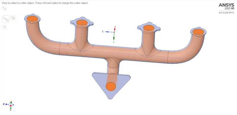
- Similarly, extract the solid volume
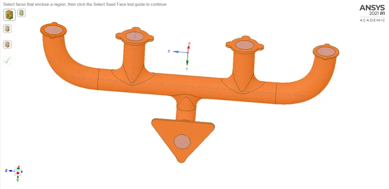
- Prepare->volume extract->select the fluid domain->rename
- The geometry is loaded to spaceclaim and the fluid and solid volumes are extracted.
-
- Workbench->share topology
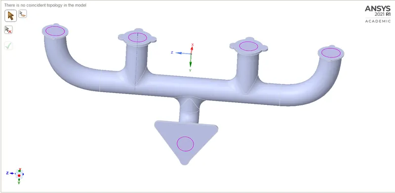
- Move the extracted components into a new component and delete the empty components
- Workbench->share topology
- MESH
- Named selection
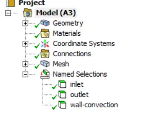
-
- Sizing
- Initially create the mesh using default element size and later could be refined. Make sure that the capture curvature is turned on.
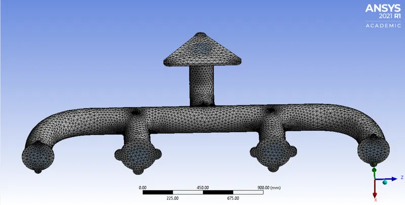
- Initially create the mesh using default element size and later could be refined. Make sure that the capture curvature is turned on.
- Inflation
- Insert->inflation (1)->select the solid domain as geometry->the fluid domain as boundary (use face selection)->first layer thickness->5mm(later changed)->update
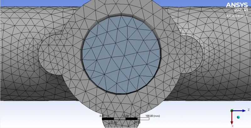
- Insert->inflation (2)->select the fluid domain as geometry->the fluid boundary as boundary (use face selection)->first layer thickness->5mm(later changed)->update
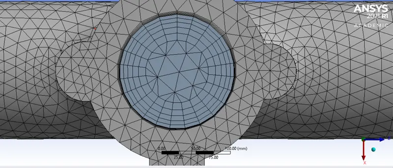
- Insert->inflation (1)->select the solid domain as geometry->the fluid domain as boundary (use face selection)->first layer thickness->5mm(later changed)->update
- Sizing
- Calculating the first layer thickness
- Characteristic length =160mm (diameter of the inlet)
- Velocity=5 m/s
- Density ρ =1.205 Kg/m3
- Dynamic viscosity µ=1.82 5-5 Kg/m-s
- Estimated y+ value =100 (for K-epsilon model, y+ ranges from 30-300) : later calculated for k-omega (y+ =3, 1<y+<5)
- Using google calculator, wall distance =5.2 mm
- SETUP
- Double precision, parallel processors-checked
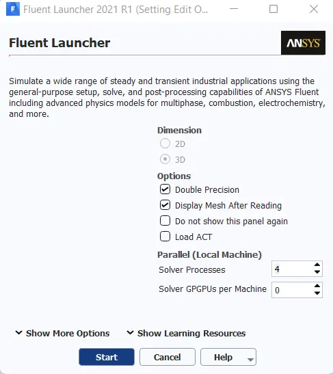
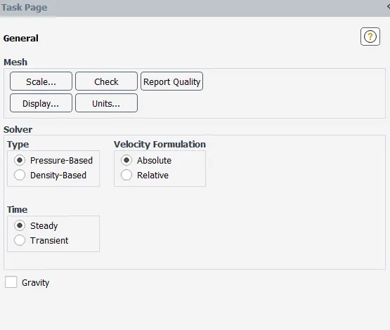
- Solver
- Density based
- Velocity foundation-absolute
- Steady flow
- Double precision, parallel processors-checked
-
- Setting up Physics
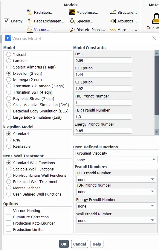
- Energy-turned on
- Viscosity-K-epsilon Turbulence model
- Setting up Physics
-
- Materials
- Fluid-air
- Solid-aluminum (both are default)
- Boundary
- Inlet- velocity 5m/s, temperature-700K
- Outlet- 0 Gauge pressure
- Wall-convection turned on- heat transfer coefficient=20W/m^2K
- Materials
- SOLUTION
- Initialization->Hybrid
- Creating contour plot
- Post-processing-contour-rename (temp-contour)->select inlet, outlet, outer wall convection and final solid geometry->select temperature->save and display
- Create animation
- Solving->activities->solution animation->velocity contour->select the view->use active->rename
- RESULTS and PLOTS
- Verification of the HTC predictions from the simulations :
The verification of the HTC prediction in the simulation can be done by using the Nusselt Number as a function of Reynold's number and Prandtl number, which is given as

During the calculation of y+, we have got Reynold's number Re=5.3e+4.
The Prandtl number, which is given by
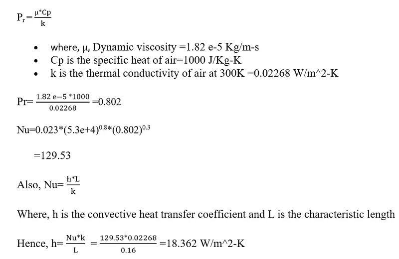
This is in great agreement with the heat transfer coefficient value that we used in simulation (20 W/m^2K)
2. Factors affecting quality of prediction.
- More the mesh refinement, better will be the results
- Proper implementation of inflation layers and boundary conditions
- Careful estimation and selection of turbulence models based on y+ value
- K-Epsilon -Default mesh
| Element Size | Default (150 mm) |
| Number of elements | 202655 |
| first layer height | 5 mm |
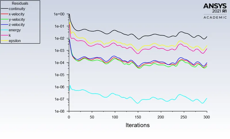
Figure 1: Residual plot for the baseline mesh
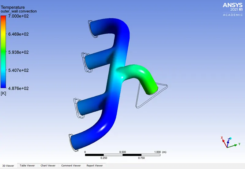
Figure 2: Temperature contour for the baseline mesh
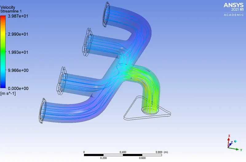
Figure 3: Streamline representation of velocity for the baseline mesh
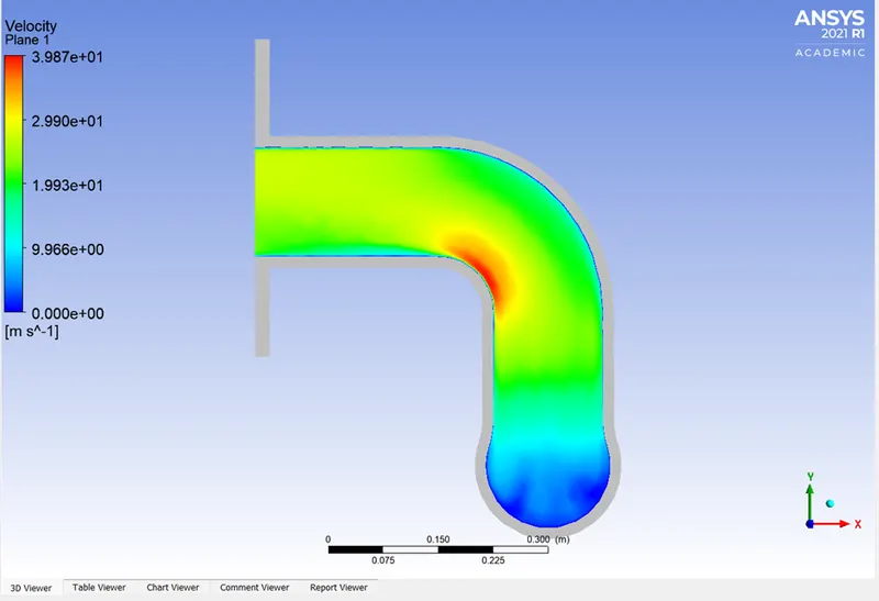
Figure 4: Velocity contour across the outlet tube for the baseline mesh
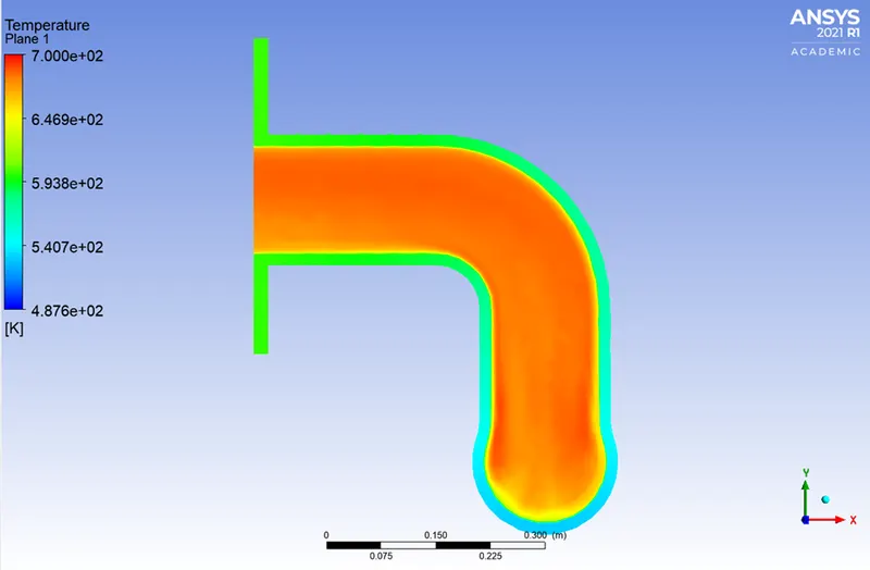
Figure 5: Temperature contour across the outlet tube for the baseline mesh
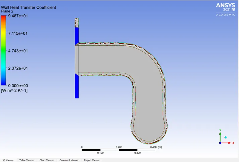
Figure 6: Surface wall heat tansfer coeffecient contour across the outlet tube for the baseline mesh
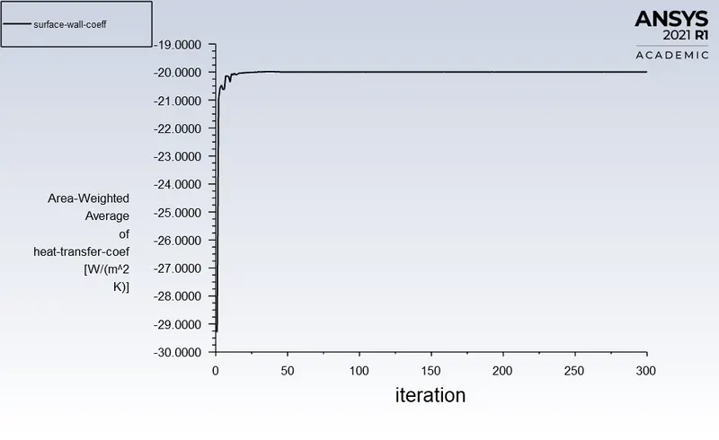
Figure 7: Surface wall heat tansfer coeffecient for the baseline mesh
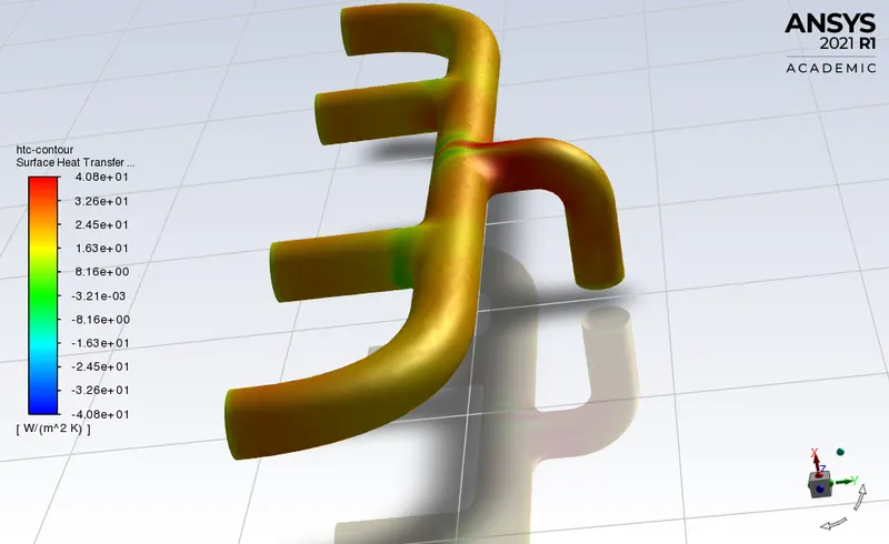
Figure 8: Surface wall heat tansfer coeffecient contour across the inflation layer for the baseline mesh
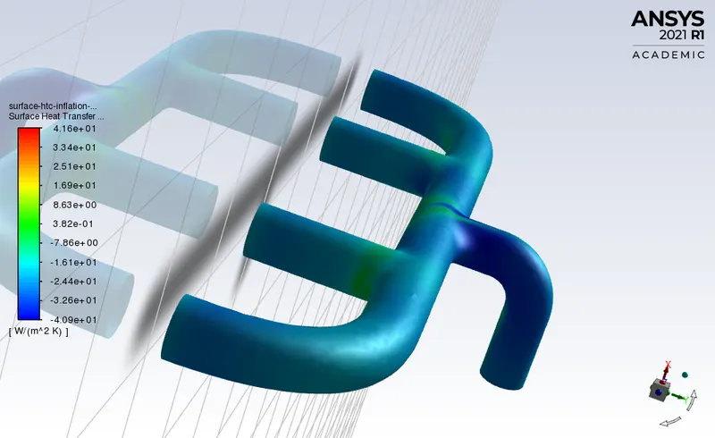
Figure 9: Surface wall heat tansfer coeffecient contour across the inflation-shadow layer for the baseline mesh
- K-Epsilon -Refined mesh (first refinement)
| Element Size | 10 mm |
| Number of elements | 334113 |
| Preferred y+ | 100 |
| first layer height | 16 mm |
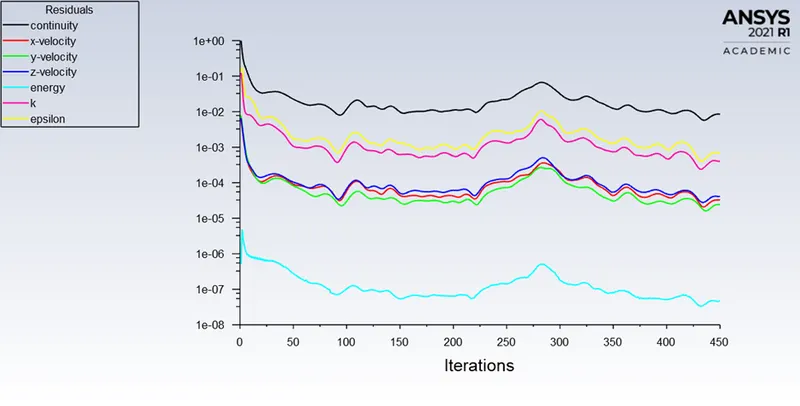
Figure 10: Residual plot for the refined mesh
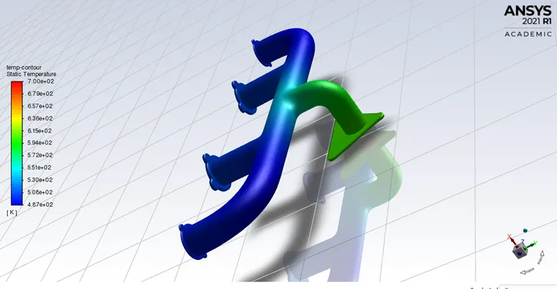
Figure 11: Temperature contour for the refined mesh
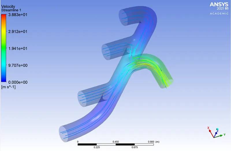
Figure 12: Streamline representation of velocity for the refined mesh
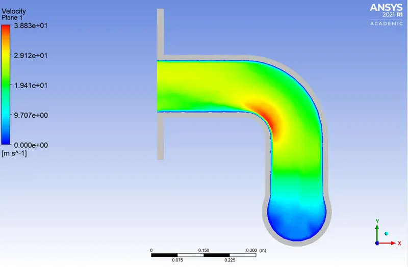
Figure 13: Velocity contour across the outlet tube for the refined mesh
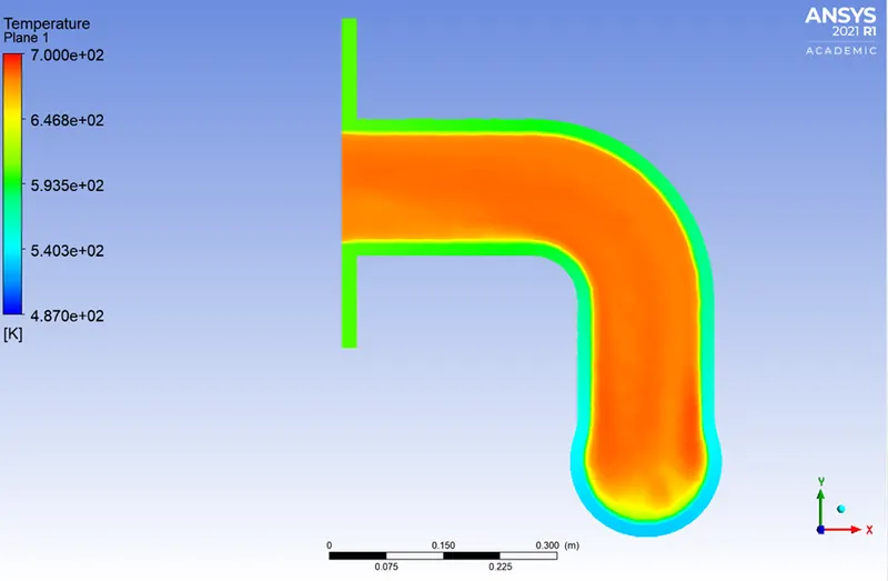
Figure 14: Temperature contour across the outlet tube for the refined mesh
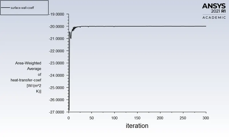
Figure 15: Surface wall heat tansfer coeffecient for the refined mesh
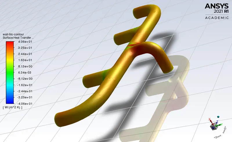
Figure 16: Surface wall heat tansfer coeffecient contour across the inflation layer for the refined mesh
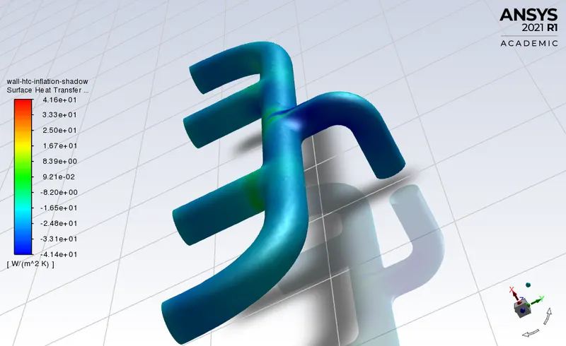
Figure 17: Surface wall heat tansfer coeffecient contour across the inflation-shadow layer for the refined mesh
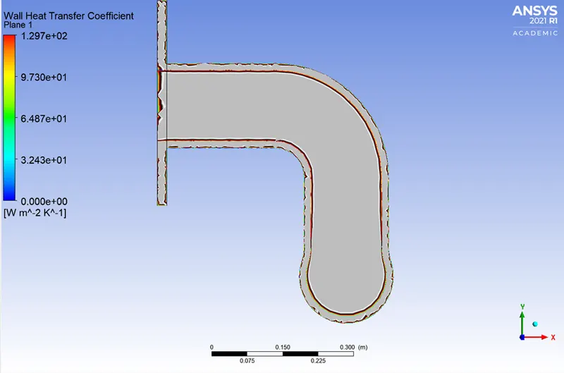
Figure 18: Surface wall heat tansfer coeffecient contour across the outlet tube for the refined mesh
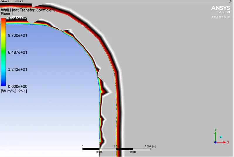
Figure 19: Surface wall heat tansfer coeffecient contour across the outlet tube for the refined mesh (zoomed)
- K-Epsilon -Refined mesh (second refinement)
| Element Size | 8 mm |
| Number of elements | 415961 |
| Preferred y+ | 100 |
| first layer height | 16 mm |
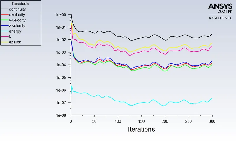
Figure 20: Residual plot for the refined mesh
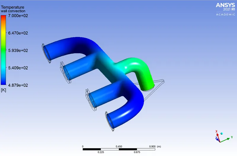
Figure 21: Temperature contour for the refined mesh
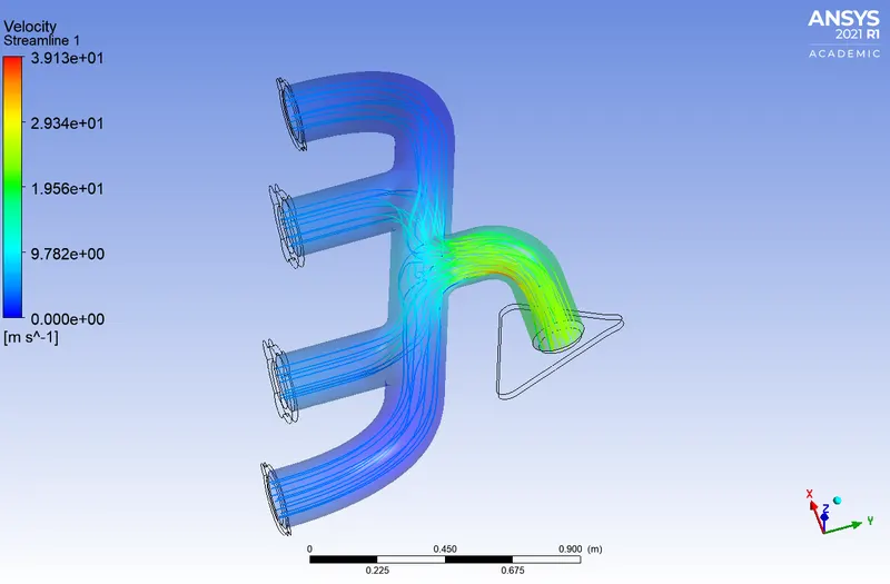
Figure 22: Streamline representation of velocity for the refined mesh
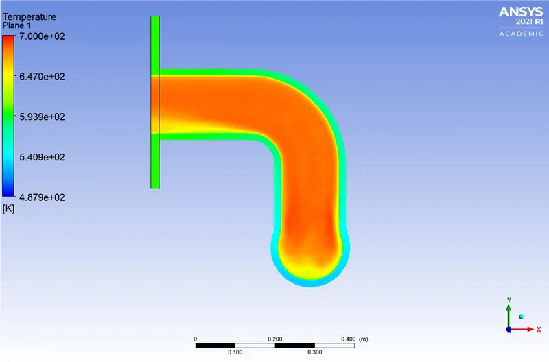
Figure 23: Temperature contour across the outlet tube for the refined mesh
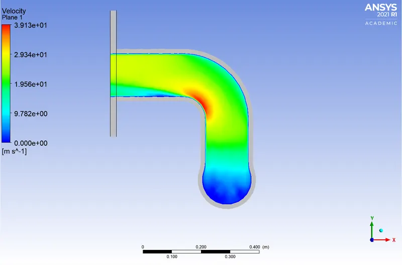
Figure 24: Velocity contour across the outlet tube for the refined mesh
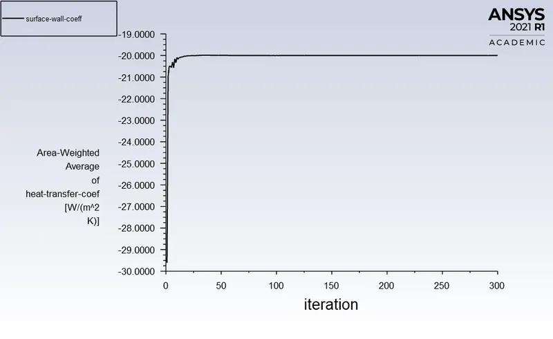
Figure 25: Surface wall heat tansfer coeffecient for the refined mesh
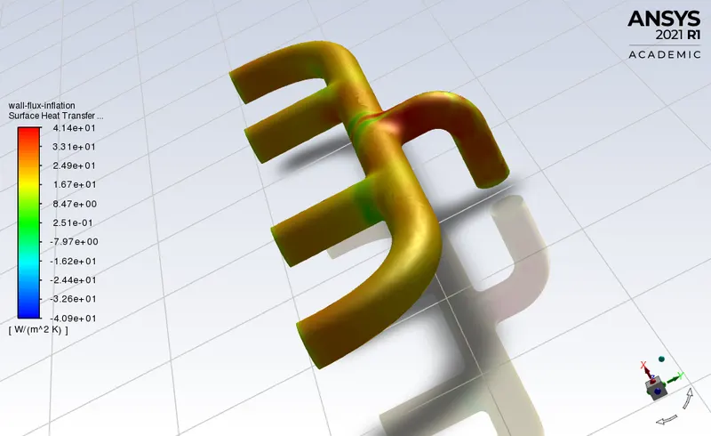
Figure 26: Surface wall heat tansfer coeffecient contour across the inflation layer for the refined mesh
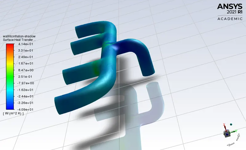
Figure 27: Surface wall heat tansfer coeffecient contour across the inflation-shadow layer for the refined mesh
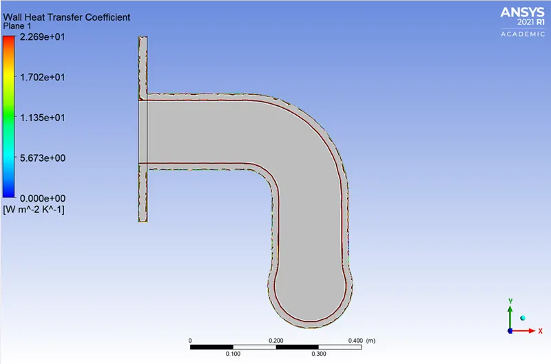
Figure 28: Surface wall heat tansfer coeffecient contour across the outlet tube for the refined mesh
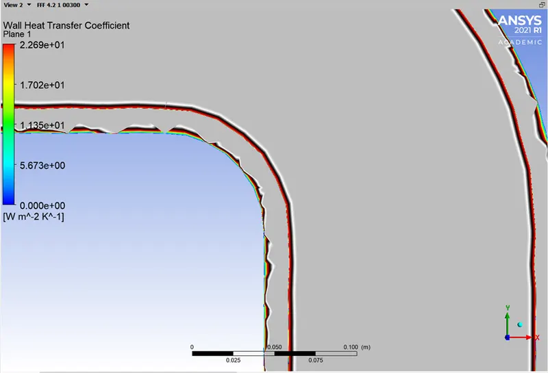
Figure 29: Surface wall heat tansfer coeffecient contour across the outlet tube for the refined mesh (zoomed)
- k-omega model-refined mesh
| Element Size | 10 mm |
| Number of elements | 397508 |
| Preferred y+ | 3 |
| first layer height | 0.16 mm |
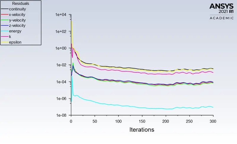
Figure 30: Residual plot for the refined mesh
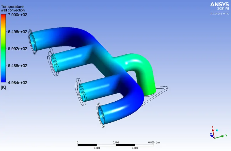
Figure 31: Temperature contour for the refined mesh
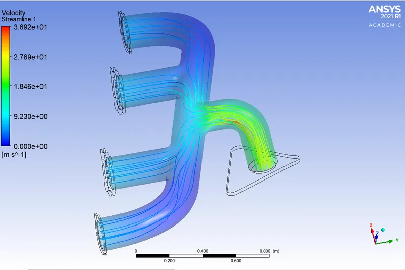
Figure 32: Streamline representation of velocity for the refined mesh
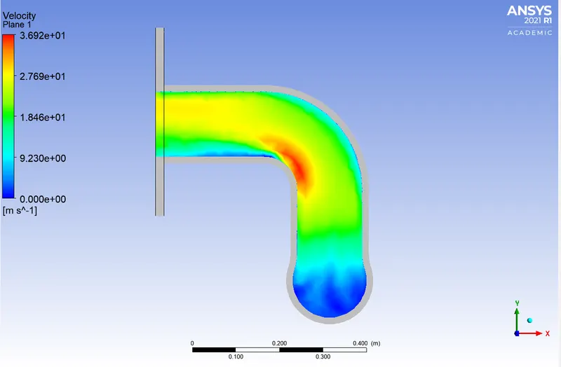
Figure 33: Velocity contour across the outlet tube for the refined mesh
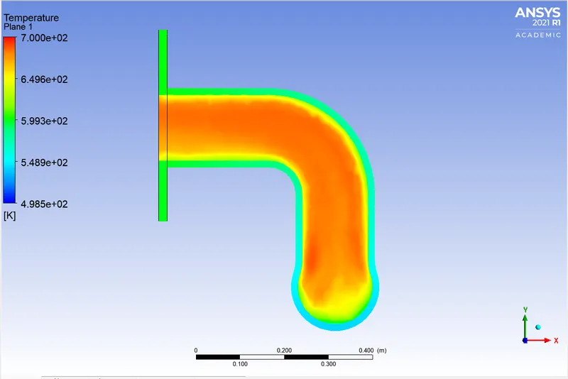
Figure 34: Temperature contour across the outlet tube for the refined mesh
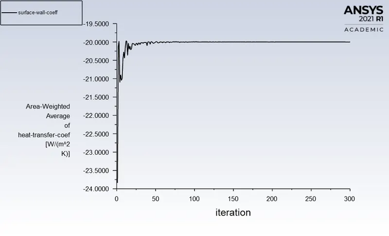
Figure 35: Surface wall heat tansfer coeffecient for the refined mesh
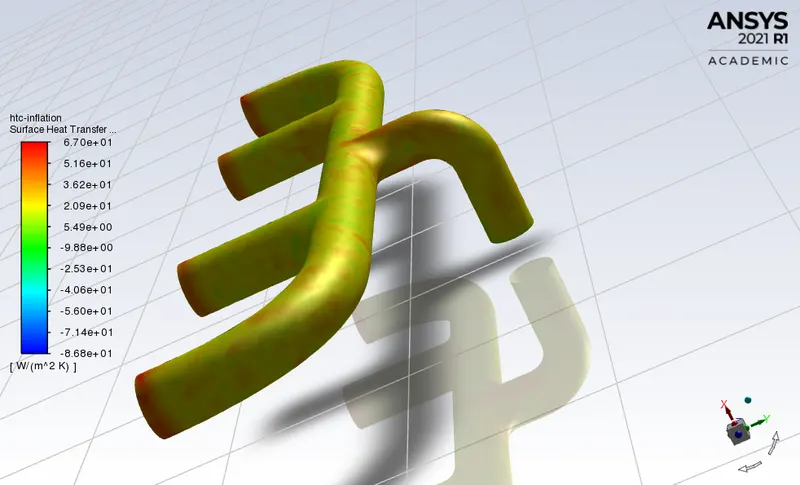
Figure 36: Surface wall heat tansfer coeffecient contour across the inflation layer for the refined mesh
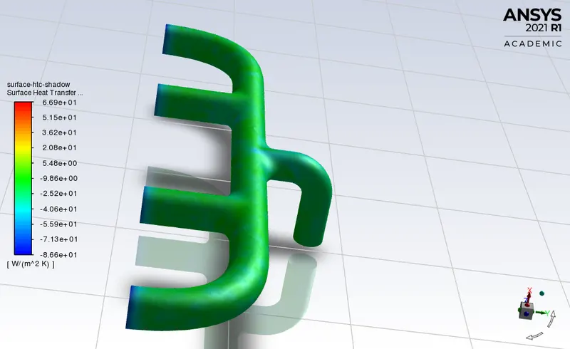
Figure 37: Surface wall heat tansfer coeffecient contour across the inflation-shadow layer for the refined mesh
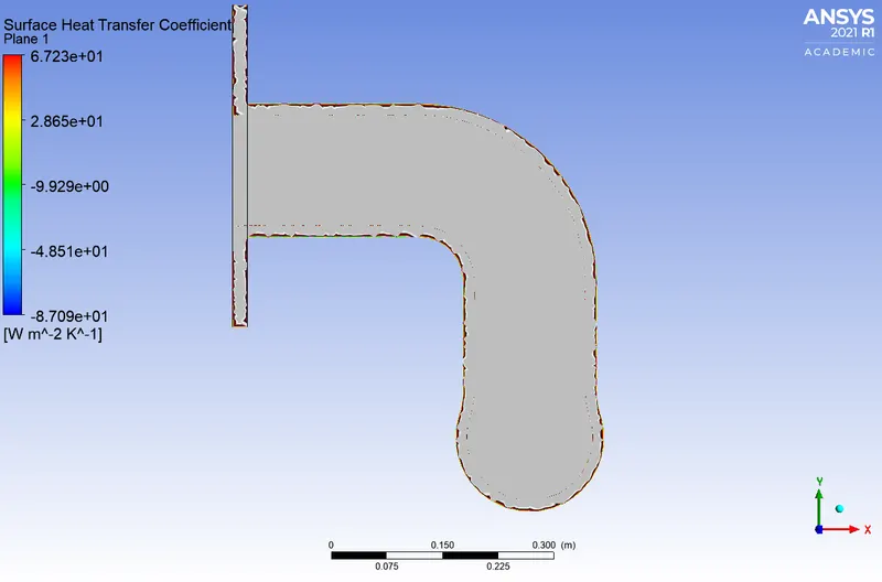
Figure 38: Surface wall heat tansfer coeffecient contour across the outlet tube for the refined mesh
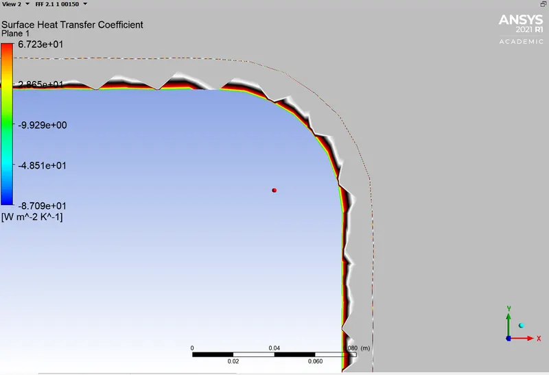
Figure 39: Surface wall heat tansfer coeffecient contour across the outlet tube for the refined mesh (zoomed)
CONCLUSION
- It can be seen that the wall heat transfer coefficient is maximum at the outlet, where the velocity is maximum. It is a bit contradictory that, even though we apply air with high temperature at the inlet fluid region, it is not reflected at the solid domain close to the inlet, but at the outlet, where all pipes meet. This is because of forced convection.
- As the air is being supplied through four inlets at same velocity, and there is only one outlet, the velocity at outlet is higher because of mass conservation. Higher the velocity, higher will be the Reynold's number and thereby higher will be the heat transfer coefficeint. Which means, more heat will be transferred from fluid to solid region at this point where the veliocity is maximum.
- For every fluid-solid interface, a shadow layer is formed by ANSYS, where one side points towards the fluid region whereas the other, towards the solid region. Comparing the contour plots of inflation and inflation shadow layers, it can be observed that the magnitude of the surface htc is almost the same, however, htc in inflation shadow layer is negative while that in inflation layer is positive. This means that the inflation shadow layer (in contact with thefluid region) is losing heat, whereas the inflation layer (in contact with the solid region) is gaining heat. Thus, there clearly exists a heat transfer from fluid to solid region.