Otto Cycle using Matlab

AIR STANDARD CYCLE

OBJECTIVE

The objective of this challenge is to program for Otto Cycle and to plot the PV diagram and also to compute its efficiency.

THEORY

Otto Cycle is considered as an ideal thermodynamic cycle which describes the basic functioning of a spark ignition (petrol) engine. It consisits of four internally reversible processes,

1-2 Isentropic compression

2-3 Constant volume heat addition

3-4 Isentropic expansion

4-1 Constant volume heat rejection

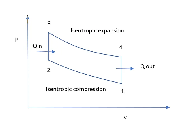
Figure 1: P-V diagram of Otto Cycle

A stroke is defined as the motion of the piston cylinder to the top dead center(TDC) or to the bottom dead center(BDC). Otto Cycle has four strokes, which begins with an intake stroke, where the reactants (fuel and air)are taken inside due to the downward motion of the piston cylinder. During the second stroke, the piston moves from BDC to TDC,significantly reducing the cylinder volume, thereby compressing reactants- Compression Stroke. It is then ignited and due to the effect of burning reactants, the third or expansion stroke occurs, where the piston moves from TDC to BDC. The final stroke is the exhaust stroke, where the burned products of combustion are expelled out of the cylinder, embarked by the pistion motion from BDC to TDC, and the cycle continues for the next intake stroke.

ENGINE KINEMATICS

1. Swept Volume: Volume of the cylinder defined by the bottom stroke(volume of cylinder)

   Vs=π/4*d^2*L,

   where d is the bore diameter and L is the stroke length

2. Clearance Volume: Vc=Swepth volume/(r-1)

   where r is the comression ratio, r=V1/V2=V4/V3

3. Total Volume= Clearance volume+Swept Volume

• For the first stroke, i.e, isentropic compression stage (1-2):

V1=Vs + Vc

P1 =1atm

T1 =500K

V2=Vc

For an isentropic process, P1*V1^γ=P2*V2^γ.......................(1)

Hence, P2=P1*(V1/V2)^γ =P1*r^γ

Ideal gas equation, PV=nRT

P1*V1/T1=P2*V2/T2

Hence, T2=P2*V2*T1/(P1*V1)

• For the second stroke, i.e, Constant volume heat addition(2-3):

V3=V2

T3 =2300K (given)

P3*V3/T3=P2*V2/T2

hence, P3=P2*T3/T2

• For the third stroke, i.e, isentropic expansion stage (3-4):

V4=V1

P4=P3*(V3/V4)^γ

T4=P4*V4*T3/(P3*V3)

EFFICIENCY: It is defined as the ratio of net work done to heat input.

η=Work done/Qin

η=1-(T1/T2)=1-r^(1-γ)

ERRORS AND CORRECTIONS

1. All the points were not getting plotted, instead only one point was plotted.

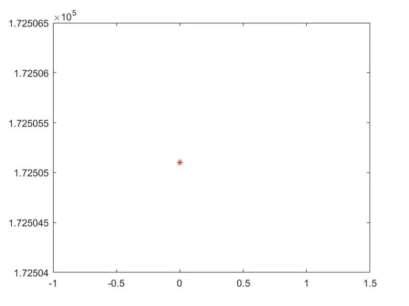
This was because of the missing 'hold on' command, hence plotting only the most recent values.

2. Error in running the function, and v_compression was not getting computed.

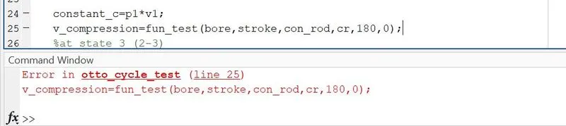
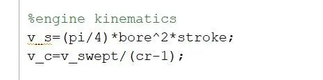
This was because the terms of swept volume were named differently in the function as shown below and was rectified once they were named similarly

3. Still V_compression was not getting computed despite showing no error in the function part. This was because, since theta is an array, element wise operator '.' was missing. Once included, this issue was also solved.

4. Despite showing no errors, the plot was not required one, showing some weird points as shown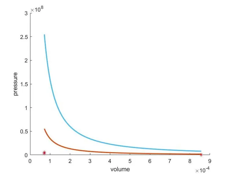

This was because the gamma term was missing while computing the constant term as shown

Once the missing term was included, the plot was perfect

FINAL CODE

function [v]=engine_kinematics_fun(bore,stroke,con_rod,cr,theta_start,theta_end)
%engine geometric parameters

pin_radius=stroke/2;
R=con_rod/pin_radius;

%engine kinematics
v_swept=(pi/4)*bore^2*stroke;
v_clear=v_swept/(cr-1);

%volume inside combustion chamber changes by
%V/Vc=1+0.5*(cr-1)[R+1-cos(theta)-((R^2-sind(theta)^2)^0.5]

%theta=linspace(0,180,180); %for one cycle
theta=linspace(theta_start,theta_end,720);%for 2 cycles

    term1=0.5*(cr-1)
    term2=R+1-cosd(theta)
    term3=(R^2-sind(theta).^2).^0.5
    v=(1+term1*(term2-term3)).*v_clear

end 

%OTTO CYCLE
clear all
close all
clc

%inputs
gamma=1.4;
t3=2300;

%engine geometric parameters
bore=0.1;
stroke=0.1;
con_rod=0.15;
cr=12;

%engine kinematics
v_swept=(pi/4)*bore^2*stroke;
v_clear=v_swept/(cr-1);

v1=v_swept+v_clear;
v2=v_clear;

%state variables at point 2 (1-2)
p1=101325;
t1=500;
%p1*v1^gamma=p2*v2^gamma (isentropic process)
p2=p1*cr^gamma;
%p1v1/t1=p2v2/t2 (ideal gas eqn)
t2=p2*v2*t1/(p1*v1);

constant_c=p1*v1^gamma; %isentropic compression process
v_compression=engine_kinematics_fun(bore,stroke,con_rod,cr,180,0);
%p_compression*v_compression^gamma=constant_c
p_compression=constant_c./v_compression.^gamma;

%state variables at point 3 (2-3)
v3=v2;
%p3v3/t3=p2v2/t2
p3=p2*t3/t2;

constant_d=p3*v3^gamma; %isentropic expansion process
v_expansion=engine_kinematics_fun(bore,stroke,con_rod,cr,0,180);
%p_expansion*v_expansion^gamma=constant_d
p_expansion=constant_d./v_expansion.^gamma;

%state variables at point 4 (3-4)
v4=v1;
%p3*v3^gamma=p4*v4^gamma (isentropic process)
p4=p3*(1/cr)^gamma;
%p3v3/t3=p4v4/t4
t4=p4*v4*t3/(p3*v3);

%thermal efficiency eta=1-(t1/t2)
eta=1-(t1/t2);

figure(1)
hold on
plot(v1,p1,'*','color','r');
plot(v_compression,p_compression,'linewidth',2);
plot(v2,p2,'*','color','g');
plot([ v2 v3 ],[ p2 p3 ],'color','b','linewidth',2)
plot(v3,p3,'*','color','k');
plot(v_expansion,p_expansion,'linewidth',2);
plot(v4,p4,'*','color','m');
plot([ v4 v1],[ p4 p1],'color','b','linewidth',2)

xlabel('volume')
ylabel('pressure')
legend('state 1','isentropic compression','state 2','constant volume heat addition','state 3','isentropic expansion','state 4','constant volume heat rejection')

RESULTS

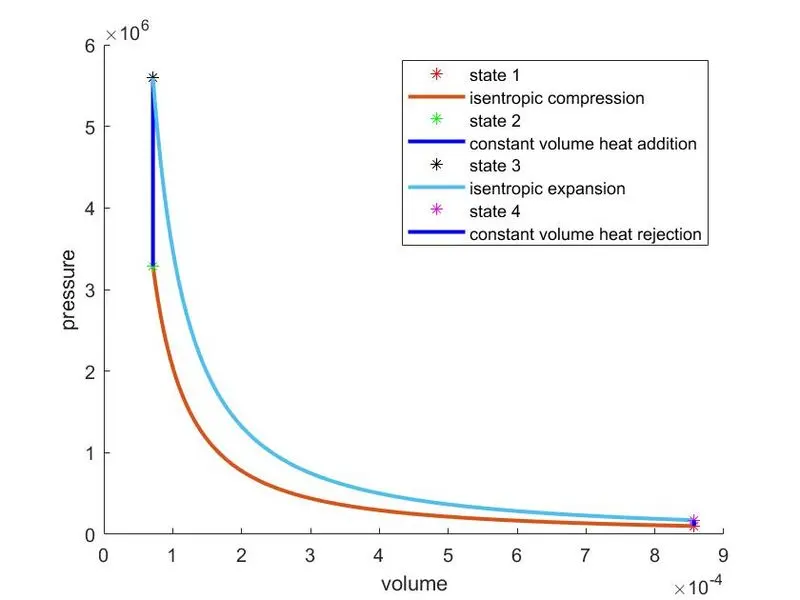
Efficiency =0.6299

The pressure-voltage diagram simulated using matlab code

CONCLUSION

The required P-V diagram of the Otto Cycle is plotted, and its efficiency is computed as 62.99%