Solving second order ODEs

SOLVING A SECOND ORDER ODE

OBJECTIVE

The challenge is to solve the second order ODE of a damped simple pendulum and to simulate its motion using Matlab.

THEORY

The ODE given was

d^2Θ/dt^2+(b/m)*dΘ/dt + (g/L)*sinΘ =0

Where b is the damping coefficient (0.05), m is the mass (1 kg), g is the acceleration due to gravity (9.81 m/s^2) and L is the length (1 m).

Solving this second order ODE using matlab requires two sets of equations, since the order is 2.

Assuming Θ=Θ1 , angular displacement……………..(1)

Then, dΘ/dt =dΘ1/dt =Θ2, angular velocity ………………………(2)

Hence, d^2Θ/dt^2 = d^2Θ1/dt^2 =dΘ2/dt , angular acceleration, which is equal to -(b/m)*dΘ/dt - (g/L)*sinΘ

i.e, dΘ2/dt = -(b/m)*Θ2 + (g/L)*sinΘ1 ………………………………(3)

hence, equations 2 and 3 are the required set of first order ODEs.

Arranging them into a 2*1 matrix Θ', such that Θ'(1)=dΘ1/dt and Θ'(2)=dΘ2/dt

Solving this will give another 2*1 matrix Θ, such that Θ(1)= Θ1 and Θ(2)=Θ2, which are angular displacement and velocity respectively

The elements of Θ’ can be written as, Θ’(1) = Θ(2)

Θ’(2) =-(b/m)*Θ(2) + (g/L)*sinΘ(1)

By writing suitable program to solve the ODE (using the ode45 function, and defining an external function), which will give the values for Θ1 and Θ2 , which are angular displacement and angular velocities respectively.

CODE

%second order ODE of SHM of a PENDULUM with damping

function [theta_dot]=odefun_second_order_SHM(t,theta)
b=0.05;
m=1;
L=1;
g=9.81;
theta1 = theta(1);
theta2 = theta(2);
theta_dot=zeros(2,1); %second order, so 2 sets of equations

theta_dot(1)=theta2;
theta_dot(2)=(-b/m)*theta2-(g/L)*sin(theta1);

end

clear all 
close all
clc

t=[0,20]; %time interval
theta0=[0,3]; %initial conditions of angular displacement and velocity

%calling the function
[t,theta]=ode45('odefun_second_order_SHM',t,theta0);

%plotting.
figure(1)
plot(t,theta(:,1),'linewidth',1);
xlabel('time');
hold on

plot(t,theta(:,2),'linewidth',1);
xlabel('time');
legend('angular displacement', 'angular velocity')
hold off

%simulating the SHM motion
n_x=length(theta);
%plotting hanging position
x0=0;
y0=0;
L=1;
ct=1;
for i=1:n_x
   y=-L*cos(theta(i,1)); %iteration is for each row element of displacement
   x=L*sin(theta(i,1));
   
   figure(2)
   %plotting the origin
   plot(x0,y0,'s','MarkerSize',10,'MarkerFaceColor','b','MarkerEdgeColor','k')
   hold on
  
   plot([x0 x],[y0 y],'k');
   hold on
   %creating the bob
   plot(x,y,'o','MarkerSize',10,'MarkerFaceColor','g','MarkerEdgeColor','k')
   xlim([-1 1]);
   ylim([-1.2 1]);
   
   hold off
   
   %capture and save the images
   M(ct)=getframe(gcf);
   ct=ct+1;
   
end
movie(M);
videofile=VideoWriter('forward_kinematics.avi','Uncompressed AVI');
open(videofile)
writeVideo(videofile,M)
close(videofile)

YOUTUBE LINK

https://youtu.be/cFTO0Tja3UQ

PLOTS

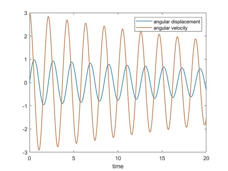
Figure 1: angular velocity and displacement vs time

RESULTS

The graphs are plotted indicate the motion of the pendulum with damping, where the angular displacement starts from 0, and the angular velocity from 3, both were the initial conditions. Over the course of time, both are reducing in amplitude because of damping effect.