Simulation of a 1D Super-sonic nozzle flow simulation using Macormack Method

OBJECTIVE

To simulate the isentropic flow through a quasi 1D subsonic-supersonic nozzle for both conservative and non-conservative forms of governing equations using the MacCormack's technique.

THEORY

Consider a steady state isentropic flow through a convergent-divergent nozzle as shown in figure 1.

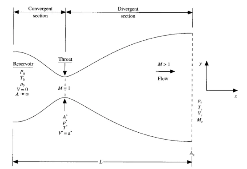
Figure 1: Schematic representation for subsonic-supersonic nozzle flow

The inlet is connected to a large reservoir, with initial parameters as pressure (Po) and temperature (To). Since the area of the reservoir is assumed to be ∞, initial velocity Vo is very small, almost 0. Also, it is a subsonic region, hence, mach number M is less than 1.The flow undergoes isentropc expansion, and reaches supersonic condition (M>1) at the exit with Pe,Te,Ve and Ae as the parameters.At the throat section, sonic flow is assumed (M=1), and hence, the flow velocity is equal to the speed of sound at this region, denoted by a∗, area A∗, pressure P∗ and temperature T∗.

There are mainly two assumptions considered in this case:

• At a given cross-sectional area A, the flow properties are uniform.
• Even though the area changes with distance x and the flow properties are 2 dimensional, we assume 1-directional flow properites, thus called as quasi-one-dimensional flow.

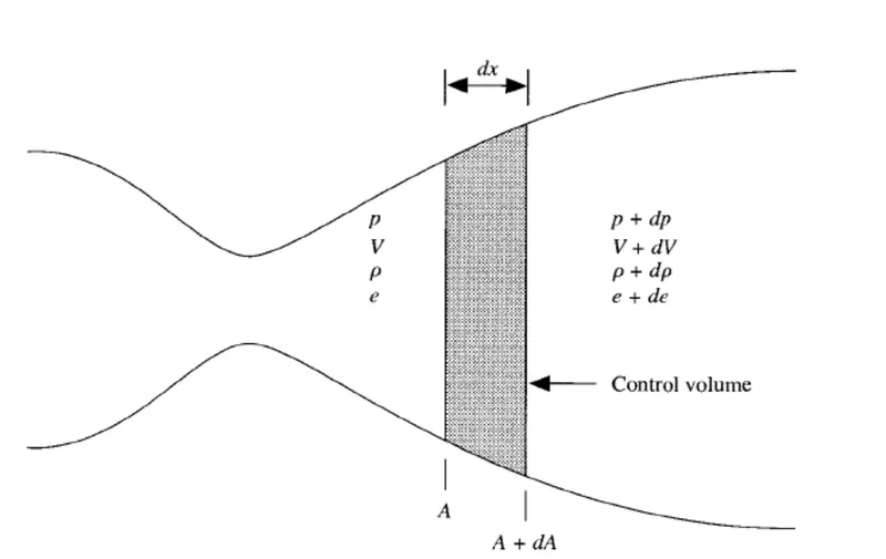
Figure 2: Control volume for deriving partial differential equations for unsteady quasi-1D-flow

Assume a small control volume with parameters as shown in figure 2.

The governing equations that define the flow are continuity, momentum and energy equations.

The NON-CONSERVATIVE FORM of governing equations, which are non-dimensional are

• continuity equation

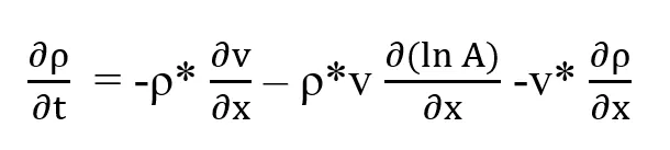
• momentum equation

• energy equation

where γ is the ratio of specefic heats Cp/Cv, and is 1.4 for standard air conditions.

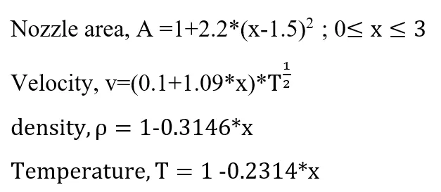
Initial conditions:

The CONSERVATIVE FORM of governing equations, which are non-dimensional are

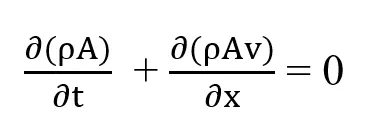
• continuity equation

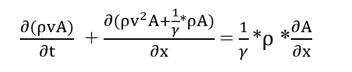
• momentum equation

• energy equation

These equations can be writtwn as

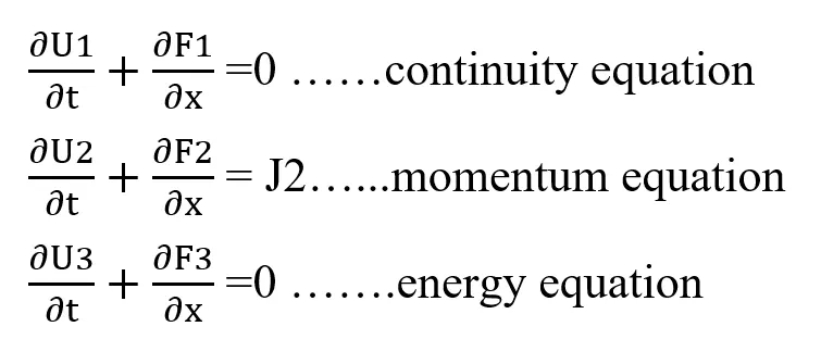
where U1,U2 and U3 are called as the solution vectors; F1,F2 and F3 are the flux vectors; and J is the source term.

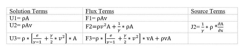
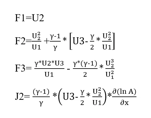
Inorder to avoid difficulties during computation and calculations, the flux vectors are represented in terms of solution vectors, i.e

F1=F1(U1,U2,U3)

F2=F2(U1,U2,U3)

F3=F3(U1,U2,U3)

J2=J2(U1,U2,U3)

where,

Initial conditions:

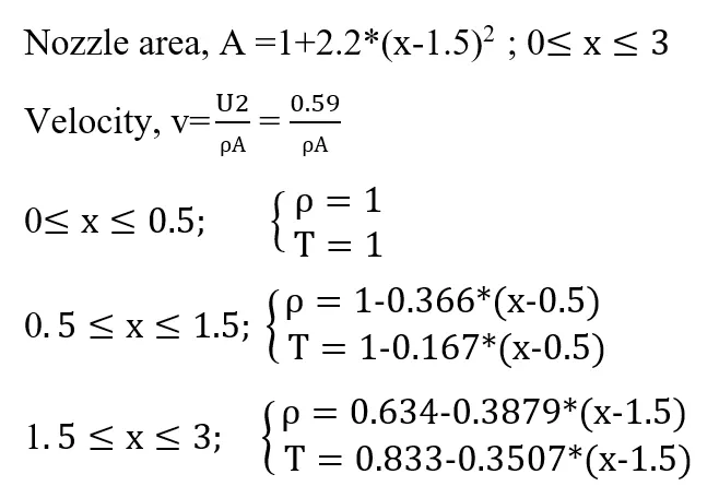
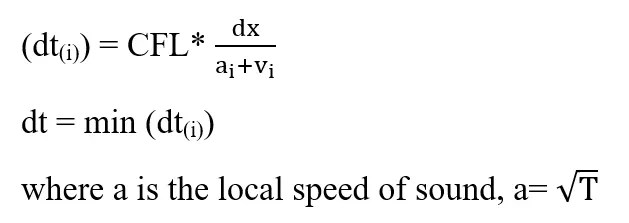
• Calculation of Time Step-Adaptive Time Step Method

These equations are solved by the MacCormack's technique.

Assume f(x) as the function to be solved. Solving this using MacCormack's technique involves

• Initial Profile : Here, certain initial assumptions are considered for the flow field variables.

• Predicted step: Forward differencing scheme is applied on the spatial terms, and obtaining the predicted derivatives.

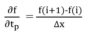
With these predicted time derivatives, we update the initial conditions.

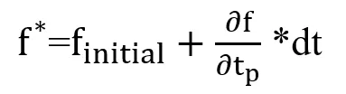
• Corrected step :Here, backward differencing is employed for the spatial terms.

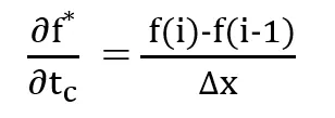
It is of immense importance to use the updated values of initial conditions from the predicted step.

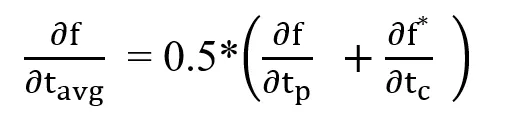
• Average step : Here, we compute the average values of time derivatives from predicted and corrected time steps.

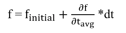
• Final Solution Update:

CODE

clear all
close all
clc

%creating x mesh
n=31;
x=linspace(0,3,n);
dx=x(2)-x(1);
throat=(n+1)/2;
A=1+2.2*(x-1.5).^2; %area
CFL=0.5;

tic;
[m_dot_throat_nc,M_throat_nc,T_throat_nc,P_throat_nc,rho_throat_nc,T_nc,M_nc,P_nc,rho_nc,v_nc,m_dot_nc]=non_conservative(n,x,dx,throat,A,CFL);
non_cons=toc;
tic
[m_dot_throat,M_throat,T_throat,P_throat,rho_throat,T,M,P,rho,v,m_dot]=conservative(n,x,dx,throat,A,CFL);
cons=toc;

%COMPARISON GRAPHS
figure(1)
hold on
plot(x,m_dot,'-*')
plot(x,m_dot_nc,'-*')
ylim([0.575 0.62])
set(gca,'YTick',(0.575:0.005:0.62))
xlabel('x')
ylabel('mass flow rate')
legend('conservative','non-conservative')
title('mass flow rate- conservative vs non-conservative')
grid on

figure(2)
hold on
plot(M_throat,'linewidth',0.95)
plot(M_throat_nc,'linewidth',0.95)
xlabel('timesteps')
ylabel('mach number')
legend('conservative','non-conservative')
title('mach number variation at throat for conservative and non-conservative')

figure(3)
hold on
plot(T_throat,'linewidth',0.95)
plot(T_throat_nc,'linewidth',0.95)
xlabel('timesteps')
ylabel('Temperature')
legend('conservative','non-conservative')
title('Temperature variation at throat for conservative and non-conservative')

figure(4)
hold on
plot(P_throat,'linewidth',0.95)
plot(P_throat_nc,'linewidth',0.95)
xlabel('timesteps')
ylabel('Pressure')
legend('conservative','non-conservative')
title('Pressure variation at throat for conservative and non-conservative')

figure(5)
hold on
plot(rho_throat,'linewidth',0.95)
plot(rho_throat_nc,'linewidth',0.95)
xlabel('timesteps')
ylabel('Density')
legend('conservative','non-conservative')
title('Density variation at throat for conservative and non-conservative')

%INDIVIDUAL GRAPHS-NON-CONSERVATIVE
figure(6)
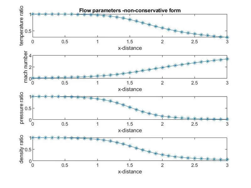
subplot(4,1,1)
plot(x,T,'-*')
xlabel('x-distance')
ylabel('temperature ratio')
title('Flow parameters -non-conservative form')
subplot(4,1,2)
plot(x,M,'-*')
xlabel('x-distance')
ylabel('mach number')
subplot(4,1,3)
plot(x,P,'-*')
xlabel('x-distance')
ylabel('pressure ratio')
subplot(4,1,4)
plot(x,rho,'-*')
xlabel('x-distance')
ylabel('density ratio')

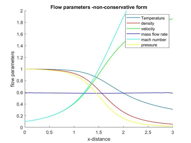
figure(7)
hold on
plot(x,T,'linewidth',0.95)
plot(x,rho,'linewidth',0.95,'color','r')
plot(x,v,'linewidth',0.95,'color','g')
plot(x,m_dot,'linewidth',0.95,'color','b')
plot(x,M,'linewidth',0.95,'color','c')
plot(x,P,'linewidth',0.95,'color','y')
xlabel('x-distance')
ylabel('flow parameters')
legend('Temperature','density','velocity','mass flow rate','mach number','pressure')
title('Flow parameters -non-conservative form')
ylim([0 2])
set(gca,'YTick',(0:0.2:2))

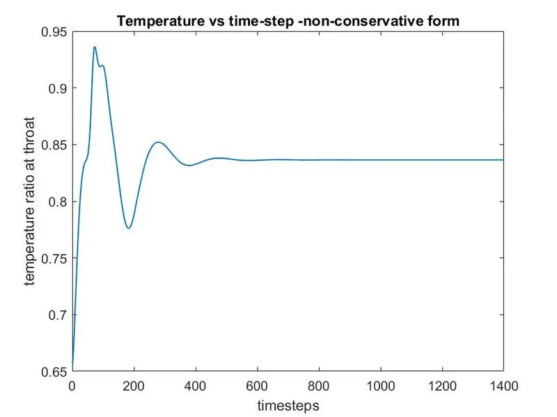
figure(8)
plot(T_throat,'linewidth',0.95)
xlabel('timesteps')
ylabel('temperature ratio at throat')
title('Temperature vs time-step -non-conservative form')

figure(9)
plot(P_throat,'linewidth',0.95)
xlabel('timesteps')
ylabel('pressure ratio at throat')
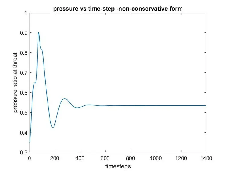
title('pressure vs time-step -non-conservative form')

figure(10)
plot(rho_throat,'linewidth',0.95)
xlabel('timesteps')
ylabel('density ratio at throat')
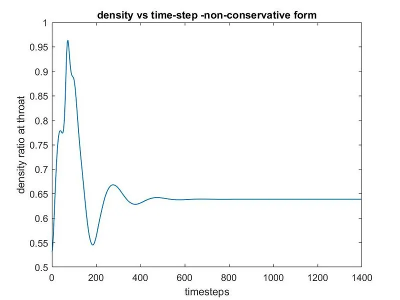
title('density vs time-step -non-conservative form')

figure(11)
plot(M_throat,'linewidth',0.95)
xlabel('timesteps')
ylabel('mach number at throat')
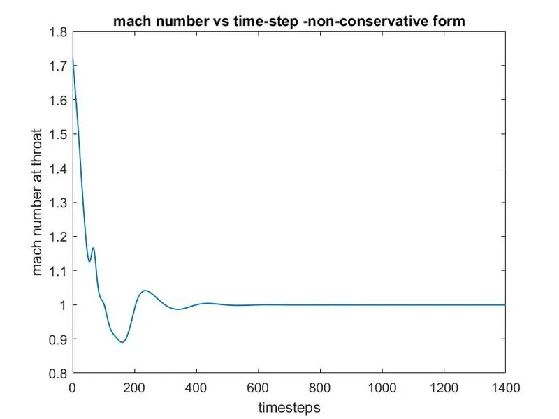
title('mach number vs time-step -non-conservative form')

figure(12)
plot(m_dot_throat,'linewidth',0.95)
xlabel('timesteps')
ylabel('mass flow rate at throat')
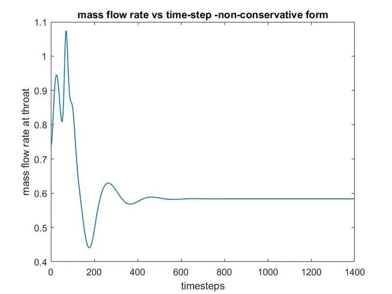
title('mass flow rate vs time-step -non-conservative form')

%INDIVIDUAL GRAPHS-CONSERVATIVE
figure(13)
hold on
plot(x,T,'linewidth',0.95)
plot(x,rho,'linewidth',0.95,'color','r')
plot(x,v,'linewidth',0.95,'color','g')
plot(x,m_dot,'linewidth',0.95,'color','b')
plot(x,M,'linewidth',0.95,'color','c')
plot(x,P,'linewidth',0.95,'color','y')
xlabel('x-distance')
ylabel('flow parameters')
legend('Temperature','density','velocity','mass flow rate','mach number','pressure')
title('Flow parameters -conservative form')
ylim([0 2])
set(gca,'YTick',(0:0.2:2))

figure(14)
plot(T_throat,'linewidth',0.95)
xlabel('timesteps')
ylabel('temperature ratio at throat')
title('Temperature vs time-step -conservative form')


figure(15)
plot(P_throat,'linewidth',0.95)
xlabel('timesteps')
ylabel('pressure ratio at throat')
title('Pressure vs time-step -conservative form')


figure(16)
plot(rho_throat,'linewidth',0.95)
xlabel('timesteps')
ylabel('density ratio at throat')
title('Density vs time-step -conservative form')


figure(17)
plot(M_throat,'linewidth',0.95)
xlabel('timesteps')
ylabel('mach number at throat')
title('Mach number vs time-step -conservative form')


figure(18)
plot(m_dot_throat,'linewidth',0.95)
xlabel('timesteps')
ylabel('mass flow rate at throat')
title('mass flow rate vs time-step -conservative form')



%NON-CONSERVATIVE FUNCTION
function [m_dot_throat_nc,M_throat_nc,T_throat_nc,P_throat_nc,rho_throat_nc,T_nc,M_nc,P_nc,rho_nc,v_nc,m_dot_nc]=non_conservative(n,x,dx,throat,A,CFL)

%calculating initial profiles as initial conditions
rho_nc=1-0.3146*x; %pressure
T_nc=1-0.2314*x; %temperature
v_nc=(0.1+1.09*x).*T_nc.^0.5; %velocity
gamma=1.4;

%calculating the time step based on cfl number
for d=1:n
    a=sqrt(T_nc(d)); %non-dimensional eqn for speed of sound
    dt_i(d)=CFL*(dx/(v_nc(d)+a));
end
dt=min(dt_i);
nt=1400; %number of iterations

%NON-CONSERVATIVE FORM
for k=1:nt %outer time loop
    %creating a copy of the initial conditions
    rho_old=rho_nc;
    v_old=v_nc;
    T_old=T_nc;
    
    %step 1: predicted  step-forward differencing for spatial terms
    for i=2:n-1
        
        %defining spatial terms
        dv_dx=(v_nc(i+1)-v_nc(i))/dx;
        drho_dx=(rho_nc(i+1)-rho_nc(i))/dx;
        dlog_A_dx=(log(A(i+1))-log(A(i)))/dx;
        dT_dx=(T_nc(i+1)-T_nc(i))/dx;
        
        %continuity equation
        drho_dt_p(i)=-rho_nc(i)*dv_dx-rho_nc(i)*v_nc(i)*dlog_A_dx-v_nc(i)*drho_dx;
        %momentum equation
        dv_dt_p(i)=-v_nc(i)*dv_dx-(1/gamma)*(dT_dx+(T_nc(i)/rho_nc(i))*drho_dx);
        %energy equation
        dT_dt_p(i)=-v_nc(i)*dT_dx-(gamma-1)*T_nc(i)*(dv_dx+v_nc(i)*dlog_A_dx);
        
        %first solution update-updating the initial conditions
        rho_nc(i)=rho_old(i)+drho_dt_p(i)*dt;
        v_nc(i)=v_old(i)+dv_dt_p(i)*dt;
        T_nc(i)=T_old(i)+dT_dt_p(i)*dt;
        
      end %predicted step end
    
    %step 2: corrected step-backward differencing for spatial terms
    for i=2:n-1
        
        %defining spatial terms
        dv_dx=(v_nc(i)-v_nc(i-1))/dx;
        drho_dx=(rho_nc(i)-rho_nc(i-1))/dx;
        dlog_A_dx=(log(A(i))-log(A(i-1)))/dx;
        dT_dx=(T_nc(i)-T_nc(i-1))/dx;
        
        %continuity equation
        drho_dt_c(i)=-rho_nc(i)*dv_dx-rho_nc(i)*v_nc(i)*dlog_A_dx-v_nc(i)*drho_dx;
        %momentum equation
        dv_dt_c(i)=-v_nc(i)*dv_dx-(1/gamma)*(dT_dx+(T_nc(i)/rho_nc(i))*drho_dx);
        %energy equation
        dT_dt_c(i)=-v_nc(i)*dT_dx-(gamma-1)*T_nc(i)*(dv_dx+v_nc(i)*dlog_A_dx);
        
    end %corrected step end
    
    %compute the average time derivative
    drho_dt_avg=0.5*(drho_dt_p+drho_dt_c);
    dv_dt_avg=0.5*(dv_dt_p+dv_dt_c);
    dT_dt_avg=0.5*(dT_dt_p+dT_dt_c);
    
    %final solution update
    for i=2:n-1
        rho_nc(i)=rho_old(i)+drho_dt_avg(i)*dt;
        v_nc(i)=v_old(i)+dv_dt_avg(i)*dt;
        T_nc(i)=T_old(i)+dT_dt_avg(i)*dt;
    end
      
    %applying boundary conditions- should be done after final solution
    %update
    
    %inlet
    v_nc(1)=2*v_nc(2)-v_nc(3);
    rho_nc(1)=1;
    T_nc(1)=1;
    
    %outlet
    v_nc(n)=2*v_nc(n-1)-v_nc(n-2);
    rho_nc(n)=2*rho_nc(n-1)-rho_nc(n-2);
    T_nc(n)=2*T_nc(n-1)-T_nc(n-2);  
    
    %finding primitive variables
    m_dot_nc= rho_nc.*A.*v_nc;      %mass flow rate
    M_nc=v_nc./sqrt(T_nc);          %mach number
    P_nc=rho_nc.*T_nc;
    
    %taking values at throat
    v_throat_nc(k)=v_nc(throat);
    rho_throat_nc(k)=rho_nc(throat);
    T_throat_nc(k)=T_nc(throat);
    P_throat_nc(k)=P_nc(throat);
    M_throat_nc(k)=M_nc(throat);
    m_dot_throat_nc(k)=m_dot_nc(throat);
    
    
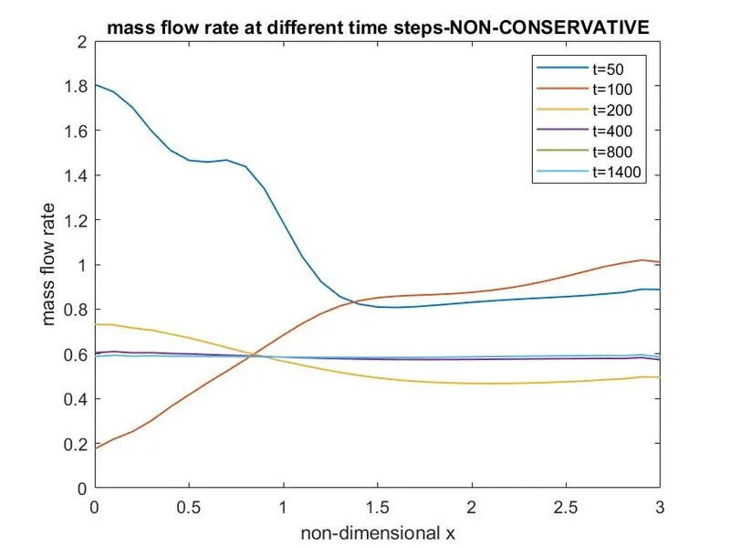
    if k==50
        figure(19)
        plot(x,m_dot_nc,'linewidth',0.95)
        hold on
    elseif k==100
        figure(19)
        plot(x,m_dot_nc,'linewidth',0.95)
        hold on
    elseif k==200
        figure(19)
        plot(x,m_dot_nc,'linewidth',0.95)
        hold on
    elseif k==400
        figure(19)
        plot(x,m_dot_nc,'linewidth',0.95)
        hold on
    elseif k==800
        figure(19)
        plot(x,m_dot_nc,'linewidth',0.95)
        hold on
    elseif k==1400
        figure(19)
        plot(x,m_dot_nc,'linewidth',0.95)
        xlabel('non-dimensional x')
        ylabel('mass flow rate')
        legend('t=50','t=100','t=200','t=400','t=800','t=1400')
        title('mass flow rate at different time steps-NON-CONSERVATIVE')
        hold on
    end
    
end

end


%CONSERVATIVE FUNCTION

function [m_dot_throat,M_throat,T_throat,P_throat,rho_throat,T,M,P,rho,v,m_dot]=conservative(n,x,dx,throat,A,CFL)
%initial conditions
for i=1:n
    if x(i)>=0 && x(i)<=0.5
        rho(i)=1;
        T(i)=1;
        
    elseif x(i)>=0.5 && x(i)<=1.5
        rho(i)=1-0.366*(x(i)-0.5);
        T(i)=1-0.167*(x(i)-0.5);
        
    elseif x(i)>=1.5 && x(i)<=3.5
        rho(i)=0.634-0.3879*(x(i)-1.5);
        T(i)=0.833-0.3507*(x(i)-1.5);
    end
end
v=0.59./(rho.*A);
m_dot=rho.*A.*v;
gamma=1.4;

%adaptive time step method
for i=1:n
    a=sqrt(T(i));
    dt_i(i)=CFL*(dx/(v(i)+a));
end
dt=min(dt_i(i));
nt=1400;

%defining the solution vectors
u_1=rho.*A;
u_2=u_1.*v;
u_3=u_1.*((T./(gamma-1))+((gamma/2)*v.^2));

%MACORMACK'S METHOD
for k=1:nt
    %predictor step
    %initialising the flux terms
    term_1=(u_2.^2./u_1);
    term_2=((gamma-1)/gamma)*(u_3-(gamma/2)*term_1);
    term_3=(gamma*u_2.*u_3)./u_1;
    term_4=0.5*gamma*(gamma-1)*u_2.^3./u_1.^2;

    F_1=u_2;
    F_2=term_1+term_2;
    F_3=term_3-term_4;
    
    %creating a copy of the solution vectors
    u_1_old=u_1;
    u_2_old=u_2;
    u_3_old=u_3;
       
    for j=2:n-1
        %defining spatial terms-forward differencing in spatial terms
        dF_1_dx(j)= (F_1(j+1)-F_1(j))/dx;
        dF_2_dx(j)= (F_2(j+1)-F_2(j))/dx;
        dF_3_dx(j)= (F_3(j+1)-F_3(j))/dx;
        
       %defining the source term-forward differencing
        dA_dx=((A(j+1))-(A(j)))/dx;
        J_2=(1/gamma).*rho(j).*T(j).*dA_dx;
        
        %continuity equation
        du_1_dt_p(j)=-dF_1_dx(j);
        %momentum equation
        du_2_dt_p(j)=-dF_2_dx(j)+J_2;
        %energy equation
        du_3_dt_p(j)=-dF_3_dx(j);
        
        %first solution update
        u_1(j)=u_1_old(j)+du_1_dt_p(j)*dt;
        u_2(j)=u_2_old(j)+du_2_dt_p(j)*dt;
        u_3(j)=u_3_old(j)+du_3_dt_p(j)*dt;
  
    end %end of predicted step
    
    %corrected step
    term_1=(u_2.^2./u_1);
    term_2=((gamma-1)/gamma)*(u_3-(gamma/2)*term_1);
    term_3=(gamma*u_2.*u_3)./u_1;
    term_4=0.5*gamma*(gamma-1)*u_2.^3./u_1.^2;

    F_1=u_2;
    F_2=term_1+term_2;
    F_3=term_3-term_4;
    
    rho=u_1./A;
    v=u_2./u_1;
    T=(gamma-1)*((u_3./u_1)-(0.5*gamma*v.^2));
    
    for j=2:n-1
        %defining spatial terms-backward differencing in spatial terms
        dF_1_dx(j)= (F_1(j)-F_1(j-1))/dx;
        dF_2_dx(j)= (F_2(j)-F_2(j-1))/dx;
        dF_3_dx(j)= (F_3(j)-F_3(j-1))/dx;
        
        %defining the source term-backward differencing
        dA_dx=((A(j))-(A(j-1)))/dx;
        J_2=(1/gamma).*rho(j).*T(j).*dA_dx;
        
        %continuity equation
        du_1_dt_c(j)=-dF_1_dx(j);
        %momentum equation
        du_2_dt_c(j)=-dF_2_dx(j)+J_2;
        %energy equation
        du_3_dt_c(j)=-dF_3_dx(j);
        
    end %end of corrected step
   
    %computing average
    du_1_dt_avg=0.5*(du_1_dt_p+du_1_dt_c);
    du_2_dt_avg=0.5*(du_2_dt_p+du_2_dt_c);
    du_3_dt_avg=0.5*(du_3_dt_p+du_3_dt_c);
    
    %final solution update
    for j=2:n-1
        u_1(j)=u_1_old(j)+du_1_dt_avg(j)*dt;
        u_2(j)=u_2_old(j)+du_2_dt_avg(j)*dt;
        u_3(j)=u_3_old(j)+du_3_dt_avg(j)*dt;
    end
    
    %initial and boundary condition
    %subsonic inflow-point 1
    u_1(1)=rho(1).*A(1);
    u_2(1)=2*u_2(2)-u_2(3);
    u_3(1)=u_1(1)*((T(1)/(gamma-1)+0.5*gamma*v(1).^2));
    
    %supersonic outflow-point n
    u_1(n)=2*u_1(n-1)-u_1(n-2);
    u_2(n)=2*u_2(n-1)-u_2(n-2);
    u_3(n)=2*u_3(n-1)-u_3(n-2);
    
    %calculating the primitive variables from solution vectors
    rho=u_1./A;
    v=u_2./u_1;
    T=(gamma-1)*((u_3./u_1)-(0.5*gamma*v.^2));
    P=rho.*T;
    M=v./sqrt(T);%mach number
    m_dot= rho.*A.*v; %mass flow rate
    
    %taking values at throat
    v_throat(k)=v(throat);
    rho_throat(k)=rho(throat);
    T_throat(k)=T(throat);
    P_throat(k)=P(throat);
    M_throat(k)=M(throat);
    m_dot_throat(k)=m_dot(throat);
    
     if k==50
        figure(20)
        plot(x,m_dot,'linewidth',0.95)
        hold on
    elseif k==100
        figure(20)
        plot(x,m_dot,'linewidth',0.95)
        hold on
    elseif k==200
        figure(20)
        plot(x,m_dot,'linewidth',0.95)
        hold on
    elseif k==400
        figure(20)
        plot(x,m_dot,'linewidth',0.95)
        hold on
    elseif k==800
        figure(20)
        plot(x,m_dot,'linewidth',0.95)
        hold on
    elseif k==1400
        figure(20)
        plot(x,m_dot,'linewidth',0.95)
        xlabel('non-dimensional x')
        ylabel('mass flow rate')
        legend('t=50','t=100','t=200','t=400','t=800','t=1400')
        title('mass flow rate at different time steps-CONSERVATIVE')
        hold on
    end
        
end  
end

PLOTS

• NON-CONSERVATIVE FORM

• CONSERVATIVE FORM

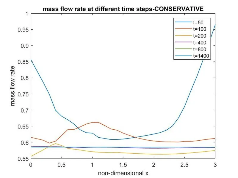
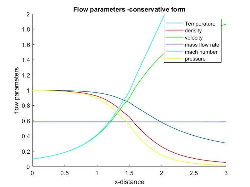
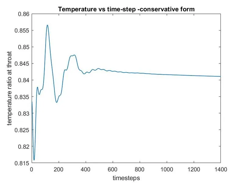
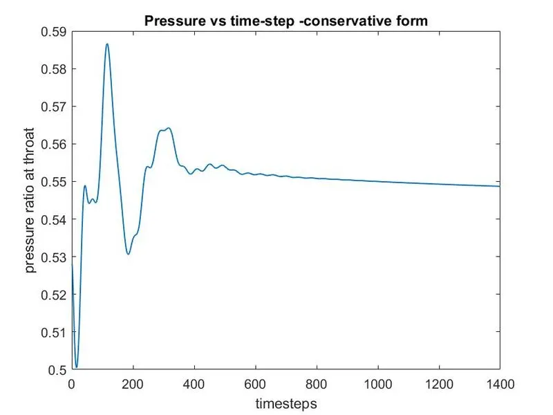
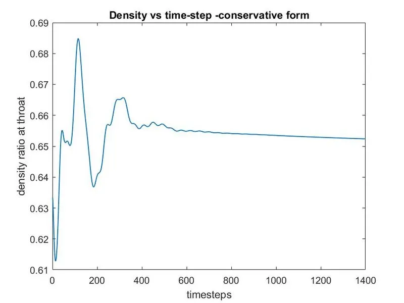
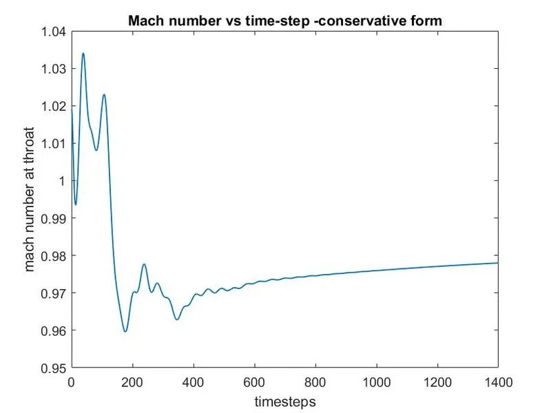
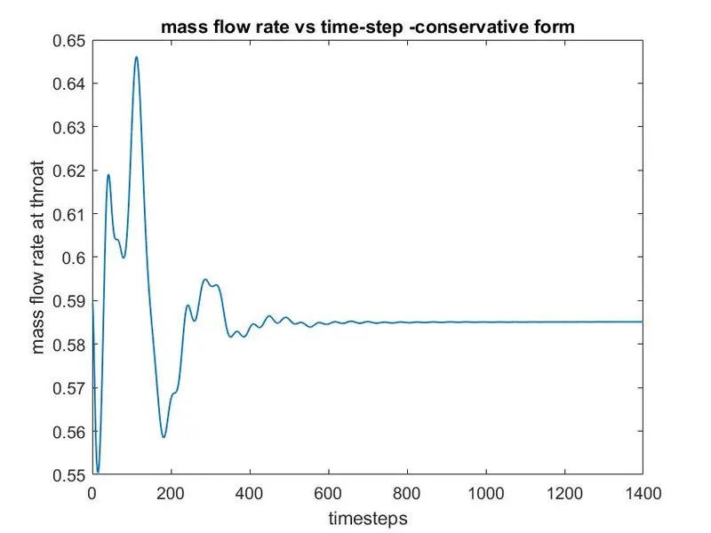
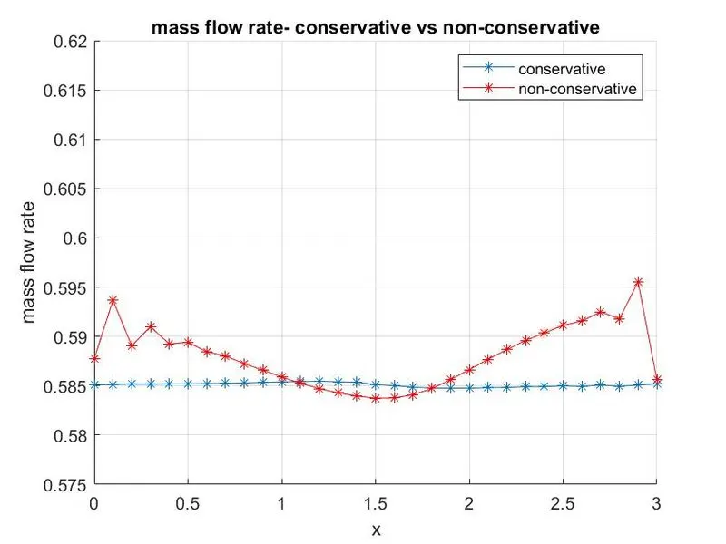
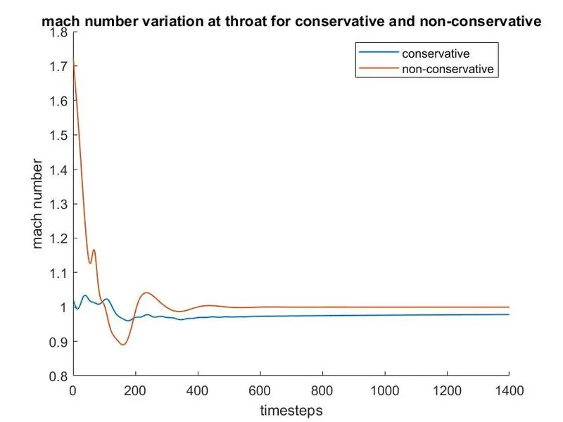
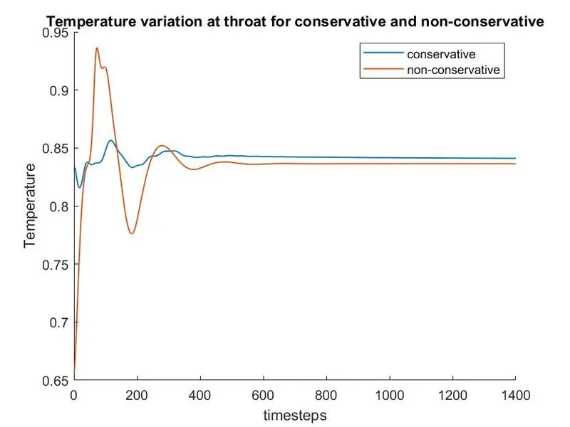
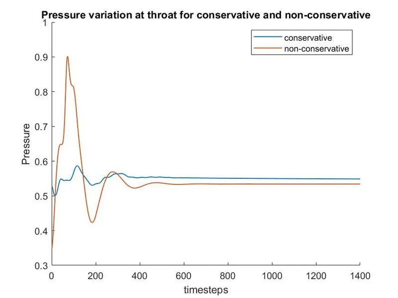
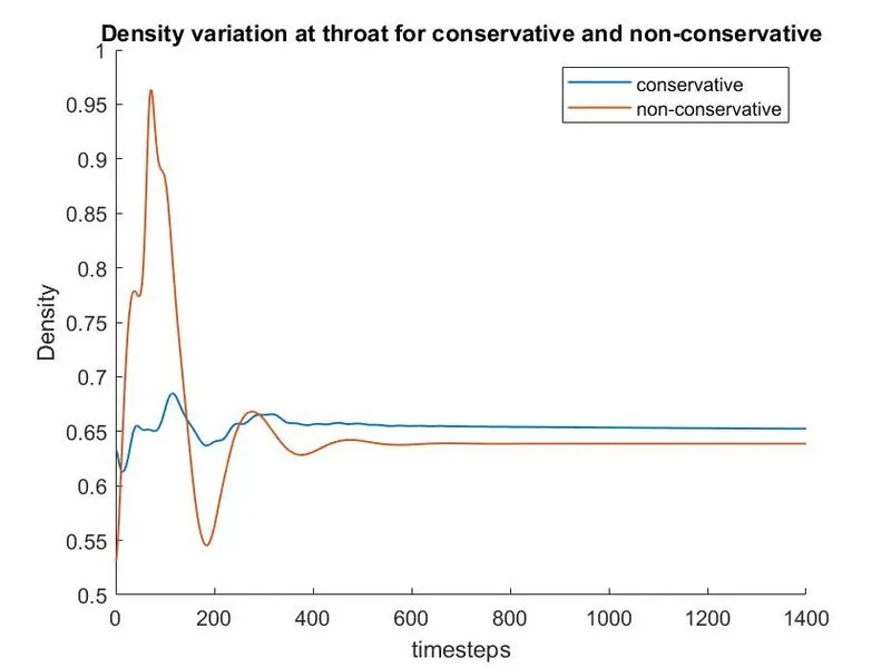
• COMPARISON OF CONSERVATIVE AND NON-CONSERVATIVE FORM

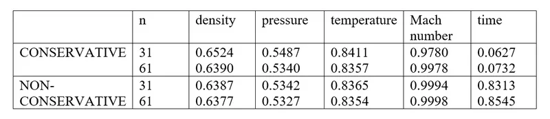
• Grid Dependency Test

Here, the grid points are varied and the flow parameters (non-dimensional) at the throat are compared along with the computation time.

• CFL Number Dependency Test

CONCLUSION

• The flow parameters in non-conservative form become constant after the 600th time step, whereas the same occur in conservative form after the 800th time step
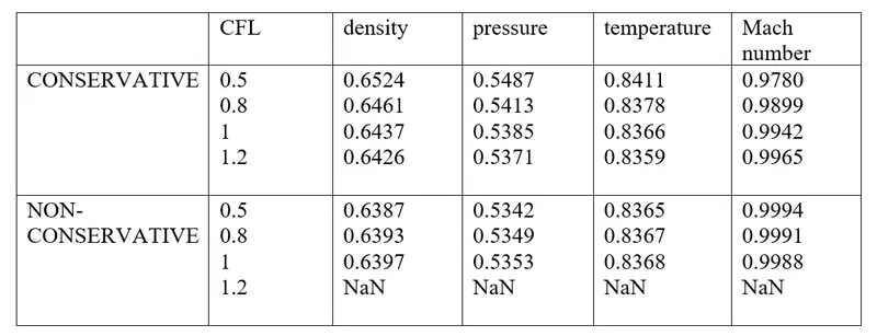
• It can be seen from the CFL number test that,CFL number doesn't have a significant impact on conservative form, whereas, in non-conservative form, the parameter values increases with CFL number, howerver, the solution blows-off when it hits 1.2
• The time taken for conservative form is lesser than that of non-conservative form

REFERENCES

[1] Andereson, John D,"Computational Fluid Dynamics the basics with applications"