Solving the steady and unsteady 2D heat conduction problem

SOLVING STEADY AND UNSTEADY 2-D HEAT CONDUCTION PROBLEM

OBJECTIVE

The primary objective of this task is to conduct a steady state and transient state analysis of a 2D heat conduction equation by using the point iterative techniques.

TASK DESCRIPTION

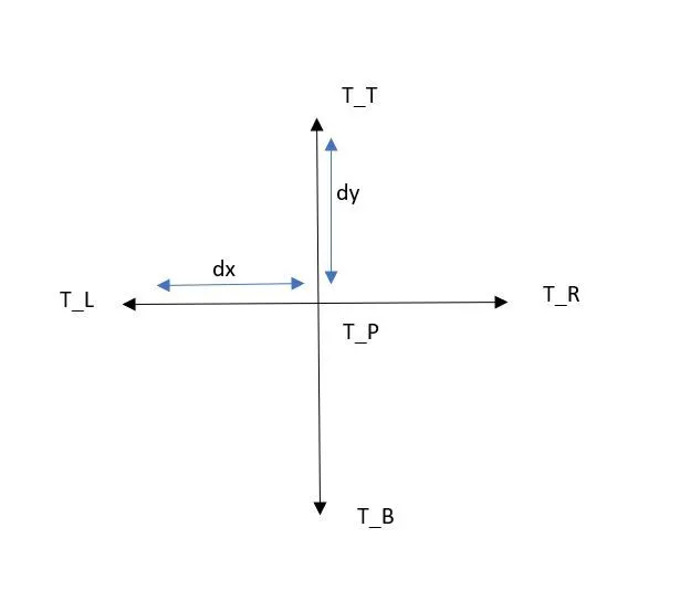
A unit square grid of 10 grid points, with boundary conditions of temperature 400K,800K,600K and 900K at left, right, top and bottom boundaries respectively are given. An initial temperature of 300K is specified inside the grid (except the boundaries).

T_L=400K

T_R=800K

T_T=600K

T_B=900K

The steady state equation has to be solved implicitly, whereas the transient state has to be solved both explicitly and implicitly. Solving an equation implicitly employs three iteration techniques:

1. Jacobi Iteration
2. Gauss Siedel Iteration
3. Successive over Relaxation Iteration

THEORY

Heat equation is a partial differential equation which describes the change/distribution of a quantity with time, within a domain, as the quantity moves according to the gradient(i.e, from higher region to lower region). It is of the form

, where u is a function of (x,y,z,t).

There are two types of heat conduction: Transient and steady state heat conduction.

Transient conduction is the period where the temperature changes with time at any place in the domain. It is also called as non-steady state conduction, signifying its temperature dependence.

The 3D transient heat conduction is given by

where α is a real coeffecient, that represents the diffusivity of the medium.

Steady state conduction occurs when the temperature difference, that acts as the driving force of conduction, is a constant. In other words, the derivatives of temperature with respect to time is zero, hence,

BOUNDARY CONDITIONS REPRESENTATION

DISCRETIZATION

The heat conduction equation is a PDE and must be discretized so as to solve it.

STEADY STATE:

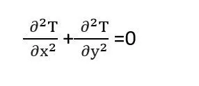
Upon discretization,

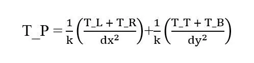
where,

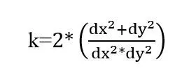
For solving the equation implicitly using:

• Jacobi Iteration, the equation can be written as

• Gauss-Siedel Iteration, the equation can be written as

• Successive over Relaxation Iteration, the equation can be written as

where, ω is the relaxation factor.

If ω >1, over relaxation

ω<1, under relaxation

TRANSIENT STATE:

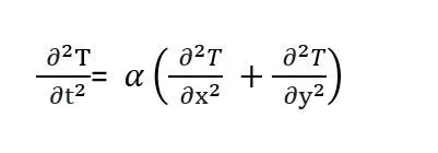
Upon discretization,

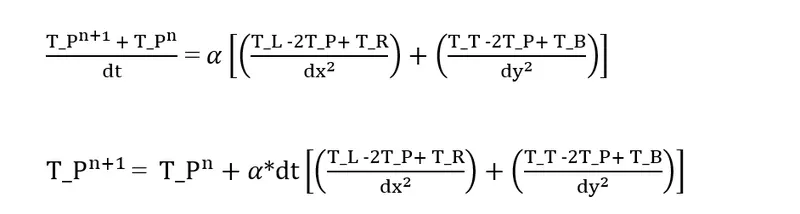
where, α is the thermal diffusion.

To solve this explicitly, no iterative techniques are needed, since all the values are known. Hence,

k1 and k2 are the CFL numbers along x and y directions respectively.

In the case of explicit diffussion processes, the total CFL number should be less than or equal to 0.5, otherwise, the solution becomes unsteady.

For solving the equation implicitly

After rearranging,

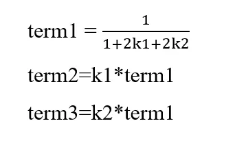
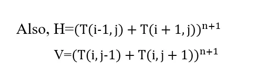
• Jacobi Iteration, the equation can be written as

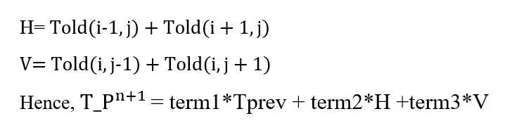
• Gauss-Siedel Iteration, the equation can be written as

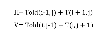
• Successive over Relaxation Iteration, the equation can be written as

CODE

• Steady State Heat Conduction-IMPLICIT

%challenge 5.1
%2d STEADY STATE heat conduction equation 
%d^2T/dx^2+d^2T/dy^2=0

clear all 
close all 
clc

%inputs
nx=10;
ny=nx;

%creating x and y grids
x=linspace(0,1,nx);
y=linspace(0,1,ny);

dx=x(2)-x(1);
dy=y(2)-y(1);
%boundary conditions
T_l=400;
T_r=800;
T_t=600;
T_b=900;

T_in=300; %value of T in all other points except the boundaries

T=T_in*ones(10,1)*ones(1,10); %creating a square grid of temperature
%Introducing the boundary conditions except the corners
T(2:ny-1,1)=T_l;%2nd to 9th row of first column
T(2:ny-1,ny)=T_r;%2nd to 9th row of last column column
T(1,2:nx-1)=T_t;%2nd to 9th column of first row
T(ny,2:nx-1)=T_b;%2nd to 9th column of last row

%computing corner values
T(1,1)=(T_t+T_l)/2;
T(10,1)=(T_b+T_l)/2;
T(1,10)=(T_t+T_r)/2;
T(10,10)=(T_b+T_r)/2;

error=9e9;
tol=1e-4;
k=2*(dx^2+dy^2)/(dx^2*dy^2);

Told=T;

iterantion_number=1;
%JACOBI ITERATION

if iterantion_number==1
    jacobi=1;
    while(error>tol)
        
        for i=2:nx-1
            for j=2:ny-1
                term1=(Told(i-1,j)+Told(i+1,j))/(k*dx^2);
                term2=(Told(i,j-1)+Told(i,j+1))/(k*dy^2);
                T(i,j)=term1+term2;
            end
        end
            error=max(max(abs(Told-T)));
            Told=T;
            jacobi=jacobi+1;
            
            contourf(x,y,T,'ShowText','on')
            ax = gca;
            % ax.XDir = 'reverse';
            ax.YDir = 'reverse';
            c = colorbar;
            c.Label.String = 'Temperature (K)';
            title_text=sprintf('no: of jacobi iterations=%d',jacobi);
            title(title_text);
            pause(0.03);
    end                 
end


%GAUSS SIEDEL ITERATION
if iterantion_number==2
    gauss=1;
    while(error>tol)
        for i=2:nx-1
            for j=2:nx-1
                term1=(T(i-1,j)+Told(i+1,j))/(k*dx^2);
                term2=(T(i,j-1)+Told(i,j+1))/(k*dx^2);
                T(i,j)=term1+term2;
            end          
        end
        error=max(max(abs(Told-T)));
        Told=T;
        gauss=gauss+1;
        
        contourf(x,y,T,'ShowText','on')
        ax = gca;
        % ax.XDir = 'reverse';
        ax.YDir = 'reverse';
        c = colorbar;
        c.Label.String = 'Temperature (K)';
        title_text=sprintf('no: of gauss iterations=%d',gauss);
        title(title_text);
        pause(0.03);
    end
end

%SUCCESSIVE OVER RELAXATION
omega=1.2;  %relaxation factor
if iterantion_number==3
    SOR=1;
    while(error>tol)
        for i=2:nx-1
            for j=2:nx-1
                term1=(T(i-1,j)+Told(i+1,j))/(k*dx^2);
                term2=(T(i,j-1)+Told(i,j+1))/(k*dx^2);
                T(i,j)=(1-omega)*Told(i,j)+omega*(term1+term2);
            end            
        end
        error=max(max(abs(Told-T)));
            Told=T;
            SOR=SOR+1;

            contourf(x,y,T,'ShowText','on')
            ax = gca;
            % ax.XDir = 'reverse';
            ax.YDir = 'reverse';
            c=colorbar;
            c.Label.String= 'Temperature (K)';
            title_text=sprintf('no: of sor iterations=%d',SOR);
            title(title_text);
            pause(0.03);
    end
end

2) TRANSIENT HEAT CONDUCTION-EXPLICIT

%challenge 5.1
%2d UNSTEADY/TRANSIENT STATE heat conduction equation -EXPLICIT
%d^2T/dt^2= alpha*(d^2T/dx^2+d^2T/dy^2)
clear all 
close all 
clc

%inputs
nx=10;
ny=nx;

%creating x and y grids
x=linspace(0,1,nx);
y=linspace(0,1,ny);

dx=x(2)-x(1);
dy=y(2)-y(1);
%boundary conditions
T_l=400;
T_r=800;
T_t=600;
T_b=900;

T_in=300; %value of T in all other points except the boundaries

T=T_in*ones(10,1)*ones(1,10); %creating a square grid of temperature
%Introducing the boundary conditions except the corners
T(2:ny-1,1)=T_l;%2nd to 9th row of first column
T(2:ny-1,ny)=T_r;%2nd to 9th row of last column column
T(1,2:nx-1)=T_t;%2nd to 9th column of first row
T(ny,2:nx-1)=T_b;%2nd to 9th column of last row

%computing corner values
T(1,1)=(T_t+T_l)/2;
T(10,1)=(T_b+T_l)/2;
T(1,10)=(T_t+T_r)/2;
T(10,10)=(T_b+T_r)/2;


k=2*(dx^2+dy^2)/(dx^2*dy^2);

Told=T;
dt=1e-3;
alpha=1.1;
k1=alpha*dt/dx^2;
k2=k1;
CFL=k1+k2;
nt=200; 


iteration=1;
    
    for m=1:nt
        for i=2:nx-1
            for j=2:ny-1
               term1=Told(i-1,j)-2*Told(i,j)+Told(i+1,j);
               term2=Told(i,j-1)-2*Told(i,j)+Told(i,j+1);
               T(i,j)=Told(i,j)+k1*term1+k2*term2 ;
            end
            
            Told=T;
            iteration=iteration+1;

            contourf(x,y,T,'ShowText','on')
            ax = gca;
            % ax.XDir = 'reverse';
            ax.YDir = 'reverse';
            c=colorbar;
            c.Label.String='Temperature  (K)';
            title_text=sprintf('no: of iterations=%d',iteration);
            title(title_text);
            pause(0.03);
        end
    end

3) TRANSIENT HEAT CONDUCTION-IMPLICIT

%2d UNSTEADY/TRANSIENT STATE heat conduction equation -IMPLICIT
%d^2T/dt^2= alpha*(d^2T/dx^2+d^2T/dy^2)
clear all
close all
clc

%inputs
nx=10;
ny=nx;

%creating x and y grids
x=linspace(0,1,nx);
y=linspace(0,1,ny);

dx=x(2)-x(1);
dy=y(2)-y(1);
%boundary conditions
T_l=400;
T_r=800;
T_t=600;
T_b=900;

T_in=300; %value of T in all other points except the boundaries

T=T_in*ones(10,1)*ones(1,10); %creating a square grid of temperature
%Introducing the boundary conditions except the corners
T(2:ny-1,1)=T_l;%2nd to 9th row of first column
T(2:ny-1,ny)=T_r;%2nd to 9th row of last column column
T(1,2:nx-1)=T_t;%2nd to 9th column of first row
T(ny,2:nx-1)=T_b;%2nd to 9th column of last row

%computing corner values
T(1,1)=(T_t+T_l)/2;
T(10,1)=(T_b+T_l)/2;
T(1,10)=(T_t+T_r)/2;
T(10,10)=(T_b+T_r)/2;


Told=T; %for the old iteration
Tprev=T; %for the old time step
Tinitial=T;

alpha=1.4;  %thermal diffusion
omega=1.2; %relaxation factor
dt=1e-3;
nt=1400;

k1=alpha*dt/dx^2;
k2=k1;
CFL=k1+k2;



error=9e9;
t_error=9e9;
tol=1e-4;

nt_jacobi=1;
nt_gauss=1;
nt_SOR=1;

jacobi_implicit=1;
gauss_implicit=1;
SOR_implicit=1;

%JACOBI
while(t_error>tol)
    error=9e9;
    while(error>tol)
        
        for i=2:nx-1
            for j=2:ny-1
                term1=(1+2*k1+2*k2)^-1;
                term2=k1*term1;
                term3=k2*term1;
                H=Told(i-1,j)+Told(i+1,j);
                V=Told(i,j-1)+Told(i,j+1);
                
                T(i,j)=(Tprev(i,j)*term1)+H*term2+V*term3;
            end
        end
        error=max(max(abs(Told-T)));
        Told=T;
        jacobi_implicit=jacobi_implicit+1;
        
        
    end
    t_error = max(max(abs(Tprev-T)));
    nt_jacobi=nt_jacobi+1;
    Tprev=T;
end

figure(1)
contourf(x,y,T,'ShowText','on')
ax = gca;
% ax.XDir = 'reverse';
ax.YDir = 'reverse';
c=colorbar;
c.Label.String='Temperature  (K)';
title_text=sprintf('no: of jacobi iterations=%d',jacobi_implicit);
title(title_text);
pause(0.03);

%GAUSS

T = Tinitial;
Told = Tinitial;
Tprev = Tinitial;
t_error=9e9;
while(t_error>tol)
    error=9e9;
    while(error>tol)
        
        for i=2:nx-1
            for j=2:ny-1
                term1=(1+2*k1+2*k2)^-1;
                term2=k1*term1;
                term3=k2*term1;
                H=T(i-1,j)+Told(i+1,j);
                V=T(i,j-1)+Told(i,j+1);
                
                T(i,j)=(Tprev(i,j)*term1)+H*term2+V*term3;
            end
        end
        error=max(max(abs(Told-T)));
        Told=T;
        gauss_implicit=gauss_implicit+1;
        
        
    end
    t_error = max(max(abs(Tprev-T)));
    nt_gauss=nt_gauss+1;
    Tprev=T;
end

figure(2)
contourf(x,y,T,'ShowText','on')
ax = gca;
% ax.XDir = 'reverse';
ax.YDir = 'reverse';
c=colorbar;
c.Label.String='Temperature  (K)';
title_text=sprintf('no: of gauss iterations=%d',gauss_implicit);
title(title_text);
pause(0.03);

%SOR
T = Tinitial;
Told = Tinitial;
Tprev = Tinitial;
t_error=9e9;

while(t_error>tol)
    error=9e9;
    while(error>tol)
        for i=2:nx-1
            for j=2:ny-1
                term1=(1+2*k1+2*k2)^-1;
                term2=k1*term1;
                term3=k2*term1;
                H=T(i-1,j)+Told(i+1,j);
                V=T(i,j-1)+Told(i,j+1);
                
                T(i,j)=(1-omega)*Told(i,j)+omega*(Tprev(i,j)*term1+H*term2+V*term3);
            end
        end
        error=max(max(abs(Told-T)));
        Told=T;
        SOR_implicit=SOR_implicit+1;
        
        
    end
    t_error = max(max(abs(Tprev-T)));
    nt_SOR=nt_SOR+1;
    Tprev=T;
end

figure(3)
contourf(x,y,T,'ShowText','on')
ax = gca;
% ax.XDir = 'reverse';
ax.YDir = 'reverse';
c=colorbar;
c.Label.String='Temperature  (K)';
title_text=sprintf('no: of SOR iterations=%d',SOR_implicit);
title(title_text);
pause(0.03);

GRAPHS

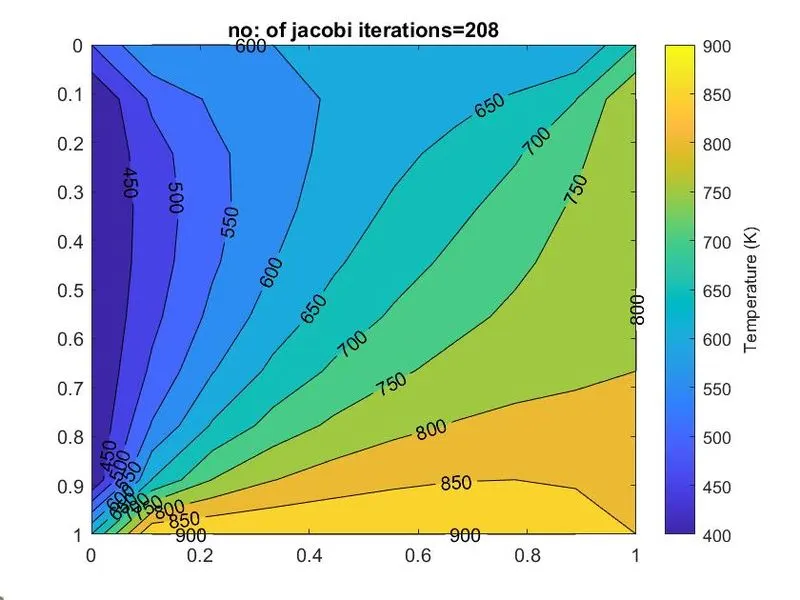
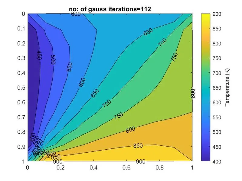
1. Steady State Heat Conduction-IMPLICIT

1) Jacobi Iteration

2) Gauss Siedel Iteration

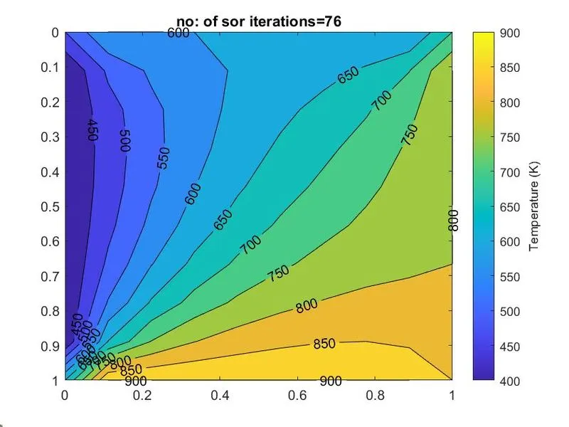
3) Successive over Relaxation Iteration

2. Transient State Analysis-EXPLICIT

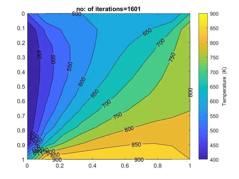
3. Transient State Analysis-IMPLICIT

1) Jacobi Iteration

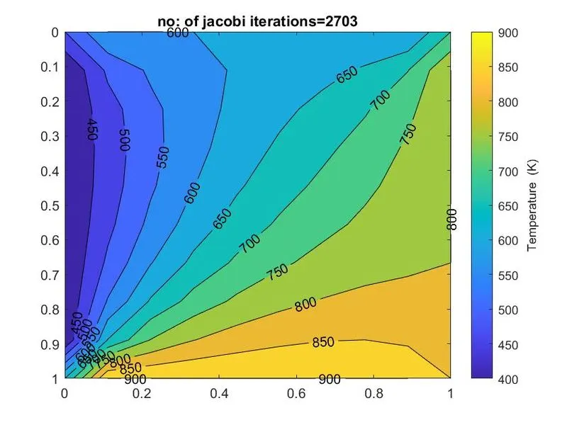
2) Gauss Siedel Iteration

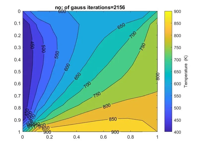
3) Successive over Relaxation Iteration

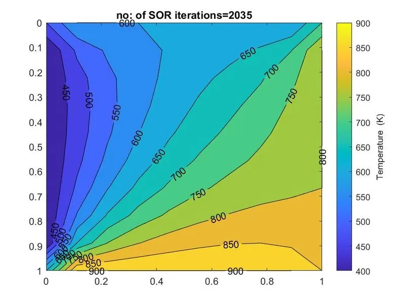
RESULTS

Scheme	Iteration Type	Number of iterations
Steady State- Implicit	Jacobi Gauss-Siedel SOR	208 112 76
Transient State-Implicit	Jacobi Gauss-Siedel SOR	2703 2156 2035
Transient State-EXplicit		1601

CONCLUSION

From the obtained results and contour plots, it can be concluded that

• the number of iterations follow the order Jacobi>Gauss-Siedel>SOR.
• among the three iterative methods, SOR is better, as the number of iterations was less than Jacobi and Gauss-Siedel, for both steady and transient states.