Week 4 - CHT Analysis on Exhaust port

Conjugate Heat-Transfer Analysis on Exhaust port

CHT analysis:-

The Conjugate Heat Transfer (CHT) analysis type allows for the simulation of heat transfer between solid and fluid domains by exchanging thermal energy at the interfaces between them.

Applications:

• simulation of heat exchangers.
• cooling of electronic equipment.
• general-purpose cooling and heating systems.

Procedure:

1. Geometry
2. Meshing
3. Setup
4. Solution
5. Results

Open Ansys Workbench and create Fluid Floe(Fluent) as a Standalone system.

Geometry:-

• Open SpaceClaim for creating Geometry.
• Import Exhaust port solid model into SpaceClaim.
• 
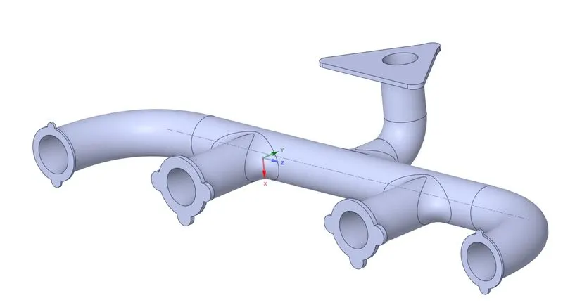
• Creating fluid domain by Volume extracting
• Fluid domain == Volume Extract => Select Edges => 4-Inlets and 1-outlet => complete(Fluid volume is extracted)
• 
• 
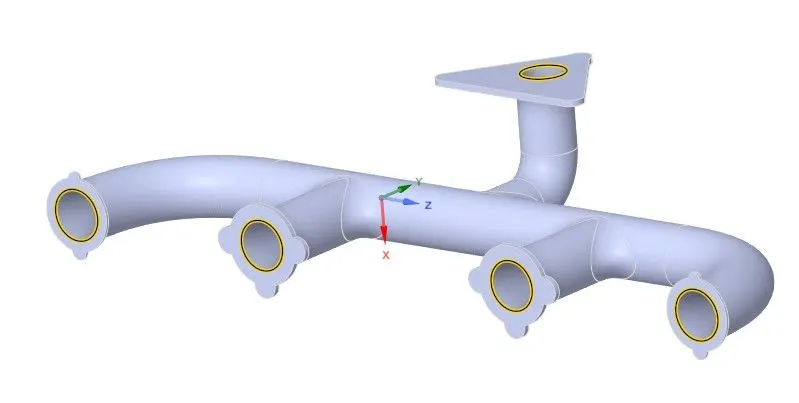
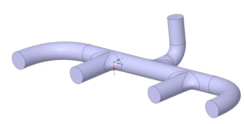
• Move Solid model and fluid domain into a new component
• 
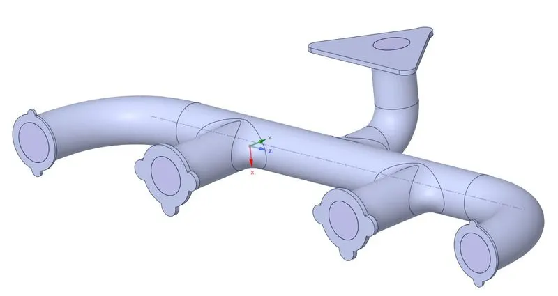
• Combined solid and fluid domains.
• At this stage Topology between solid and fluid domains has not been shared.
• So we have to share the Topology so that solution information gets shared in between those bosies
• Workbench => Share
• 
• 
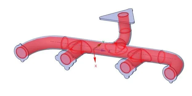
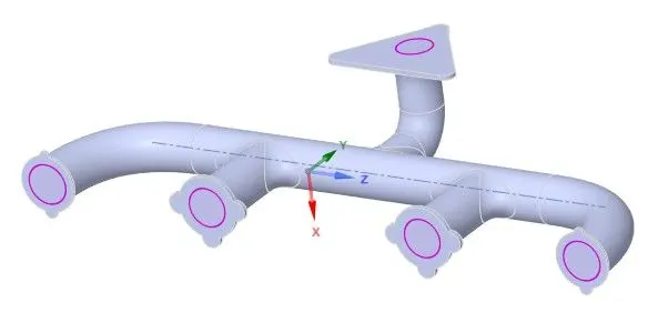
• The above pink circles indicate that Topology shared

2. Maintain the y+ value according to the turbulence model.

To capture correct turbulence we use various turbulence models but the accuracy of capturing correct results depends on various factors like element size, boundary conditions etc.

To capture effects in viscous sublayer the mesh elemet should be small enough to fit into viscous sublayer. to calculate we use Y+ method to calculate first layer thickness.

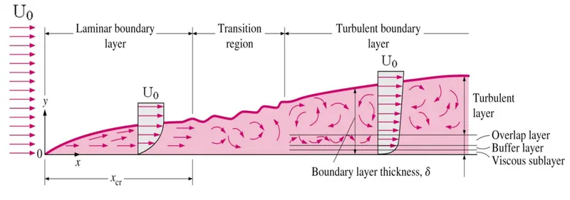
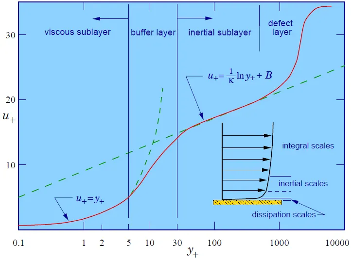
First layer thickness calculation procedure using Y+.

`text(Density of fluid (air)) = rho = 1.225 text( Kg/m^3)`

`text(Dynamic Viscosity) = mu = 1.7894*10^(-5) = text( Kg/ms)`

`text(Pipe Diameter) = D = 0.15 text( m)`

`text ( Inlet Velocity) = 5 text( m/s)`

`text ( Air Temperature) = 700 text( K)`

• `text(Reynolds number ) = R_e = (rho*V*D)/mu`
• `text ( Skin friction coefficient) = C_f`
  • `text(Laminar )= C_f = 0.664/(sqrt(R_e))`
  • `text(Turbulent )= C_f = 0.027/((R_e)^(1/7))`
• `text ( Wall shear stress) = tau_w = (C_f*rho*V^2)/2`
• `text ( Frictional velocity) = mu_f = sqrt((tau_w)/(rho))`
• `text (First Layer Thickness) = Y = (Y^+ *mu)/(mu_f*rho) text(m)`
• `text (N_th layer thickness) = Y*(text(Growth rate)^(number of layers -1))`

# Air properties
rho = 1.225 # Density Kg/m3
mu  = 1.7894e-5 # Dynamic viscosity kg/m-s
V   = 5 # Inlet Velocity m/s
D   = 0.1669 # Diameter m
y   = 4 # Y+ 

# Reynolds number 
Re = (rho*V*D)/mu
# Skin friction co-efficient
C_f = 0.027/pow(Re,1/7)
# Wall shear stress
T_w = 0.5*C_f*rho*pow(V,2)
# Frictional velocity
U_f = (T_w/rho)**0.5
# first layer thickness
Y   = ((y*mu)/(U_f*rho))*1000   # mm
print('First layer thickness = ', Y)

2. Meshing:-

• 
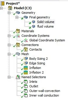
• Create Named Sections (Inlets, Outlet, Outer wall convection, inner wall conduction)
• 
• 
• 
• 
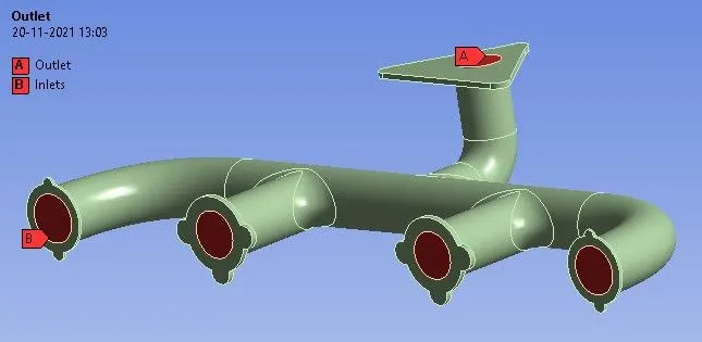
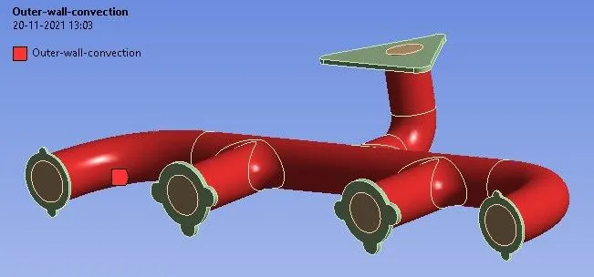
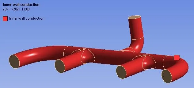
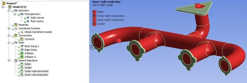
• Meshing is done by four methods
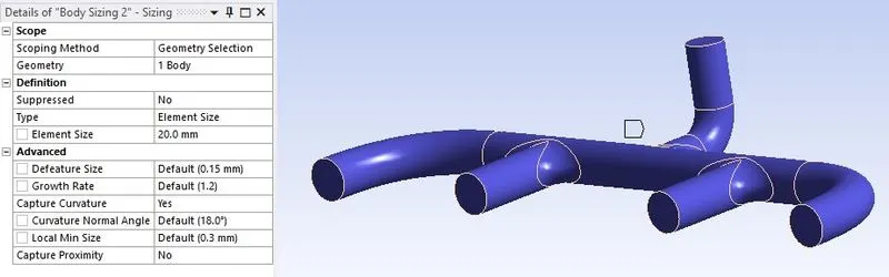
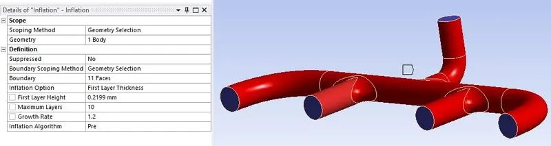
  1. Insert => Method => Geometry = Fluid domain (body) => Type Element size = 20 mm => capture Curvature => Yes
     • 
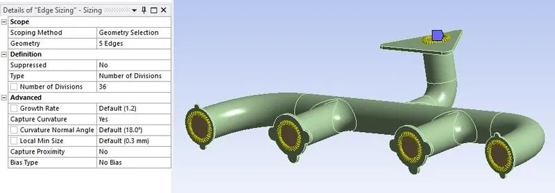
  2. Insert => Method => Geometry = Inlets & outlet edges => Number of divisions = 36 => capture Curvature => Yes
     • 
  3. Insert => Inflation => Geometry = Fluid domain => Boundary = Fluid outer wall => Option = Total thickness => N layers = 10 => Growth rate = 1.2 => First layer Thickess = 0.2199
     • 
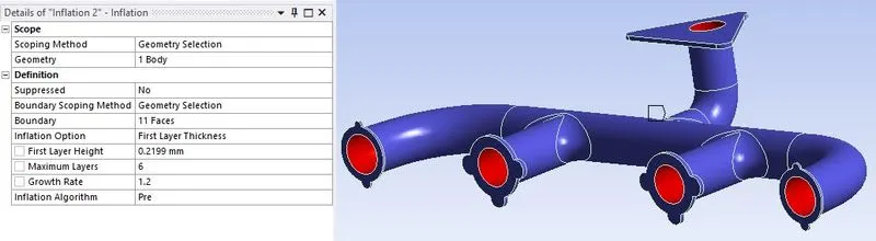
  4. Insert => Inflation => Geometry = Fluid domain => Boundary = Solid inner wall => Option = Total thickness => N layers = 6 => Growth rate = 1.2 => First layer Thickess = 0.2199
     • 
• Generate mesh
• 
• 
• 
• 
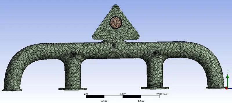
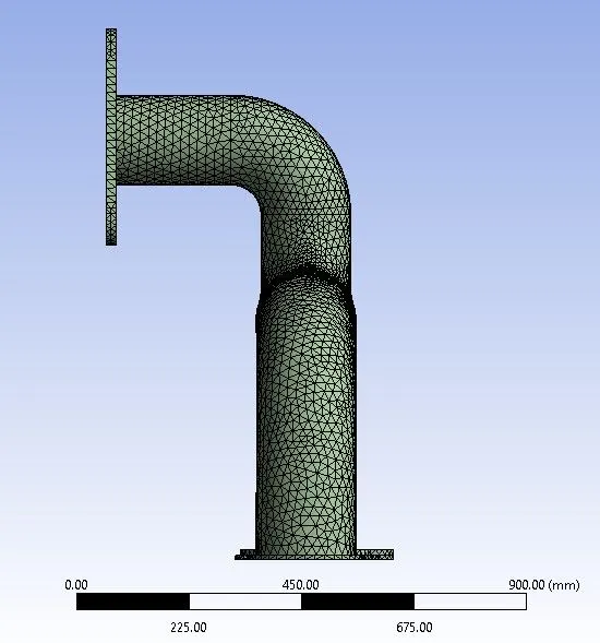
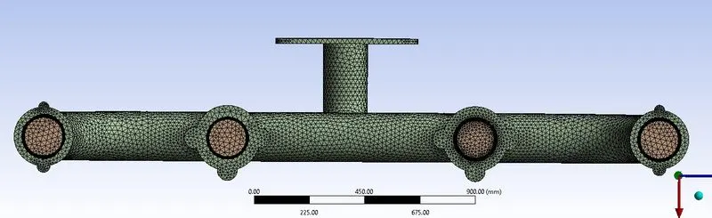
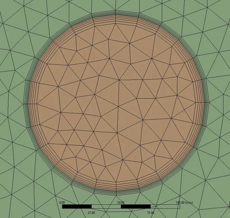
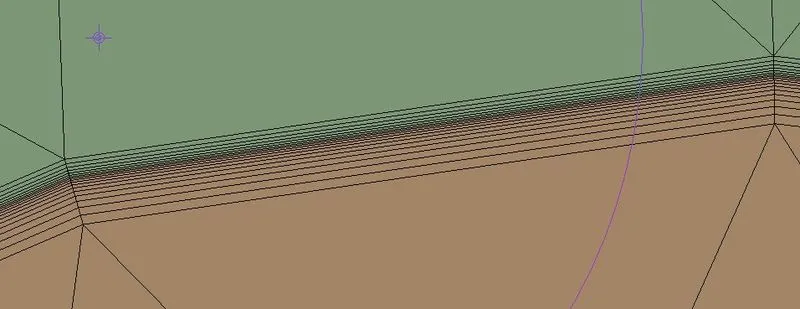
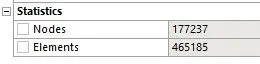
• Statistics of mesh
  • 

3 & 4. SetUp & Solution:-

• Double Presission, Solve processers = 4.
• `text(Fluid velocity)/text(Sound velocity)=5/343=0.01<0.3 text( Mach number)`
• Solver = Pressure Based, Velocity Formulation = Absolute, Time= Steady
• Energy = on
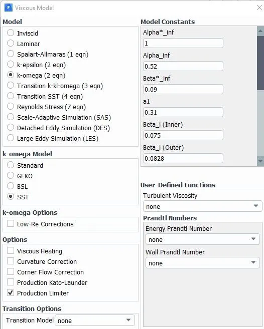
• Viscous Model = k-omega, model => SST
• 
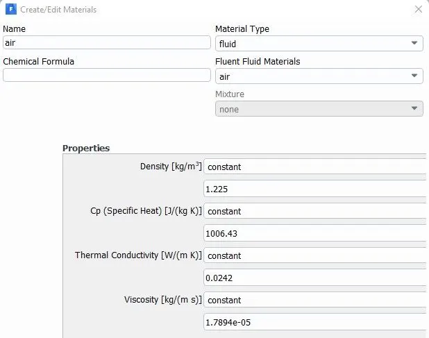
• Fluid Material => Default Air from Fluent database.
• 
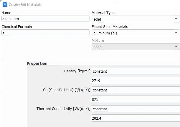
• Solid Material => Default Aluminium from Fluent database.
• 
• Cell zone conditions
  • Fluid domain = Air
  • Solid body = Aluminium
• Boundary Conditions
  • 
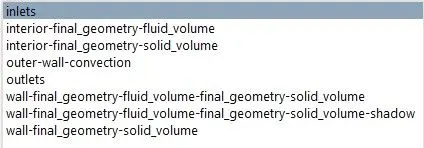
  • Inlet => Inlet Velocity & Temperature = 5m/s & 700K
  • Outlet => Pressure outlet = 0 gauge
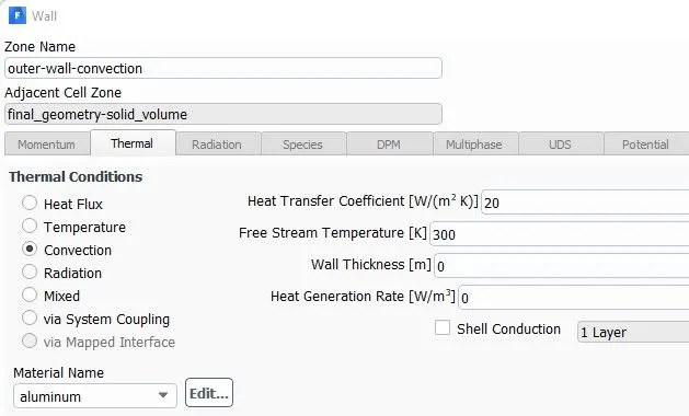
  • Outer wall convection => convection => Heat Transfer coefficient = 20 W/m^2 K
  • 
  • wall => Coupled
• Methods => Coupled Pressure velocity scheme.
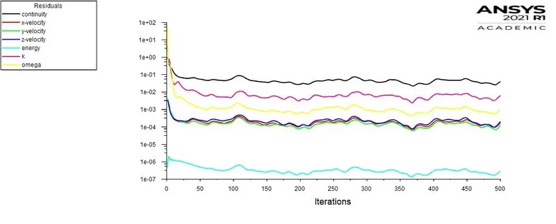
• Residual moniters = Uncheck the Convergence
• Hybrid initialization
• Run calculation for 500 iterations.
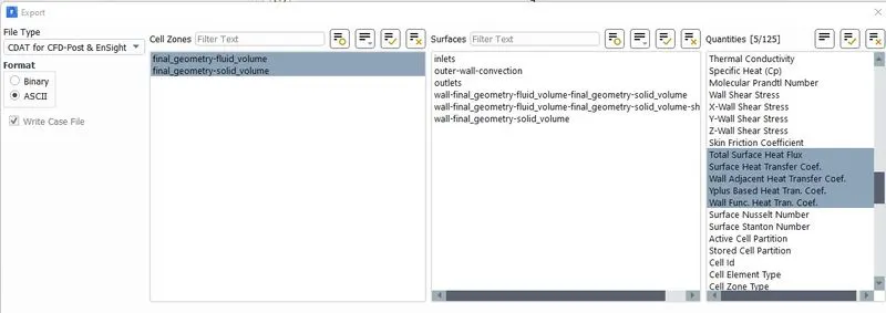
• Export results
• 

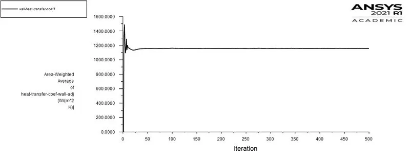
Graphs :-

• Residuals
• 
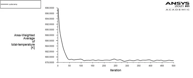
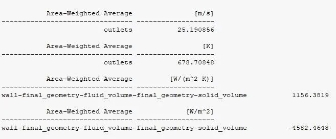
• Outlet Temperature
• 
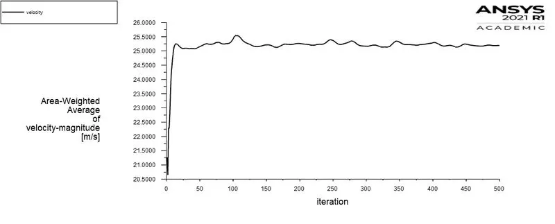
• Outlet Velocity
• 
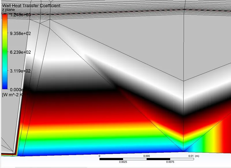
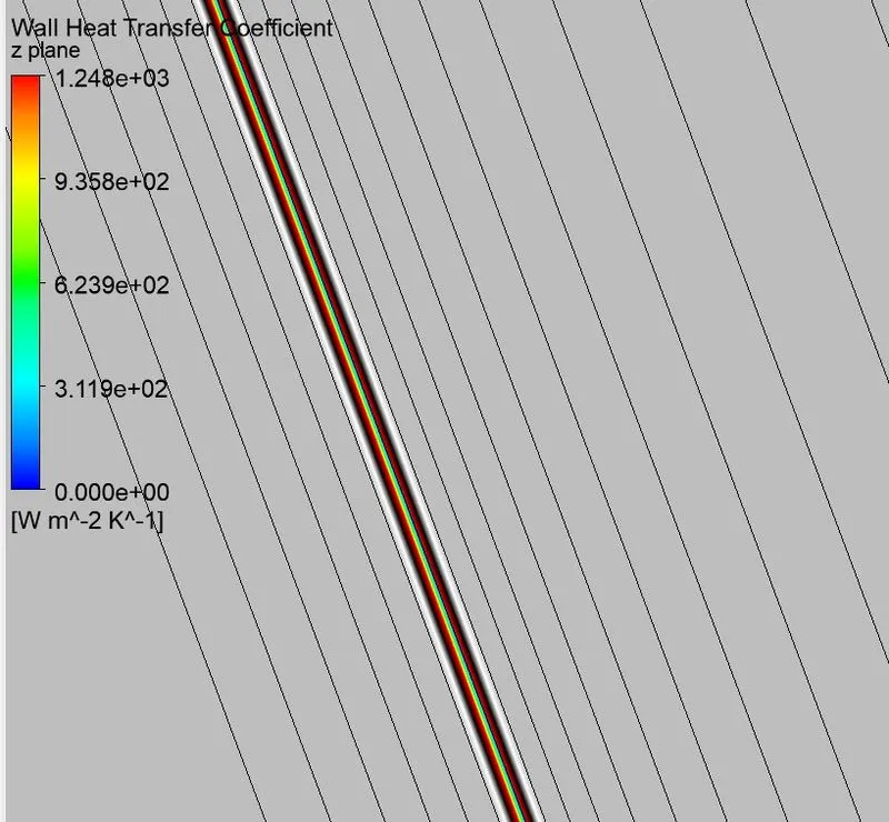
• Wall heat transfer coefficient on the fluid, Solid interface surface
• 
• Numerical solution:-
• 

Results:-

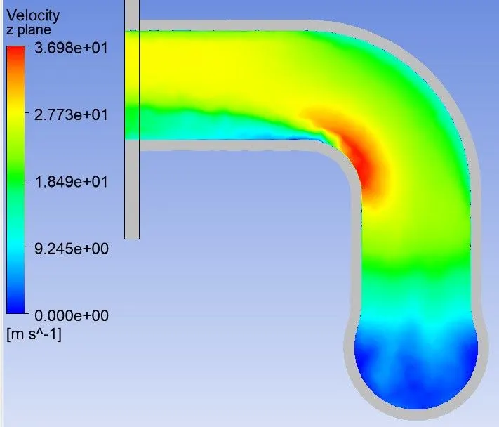
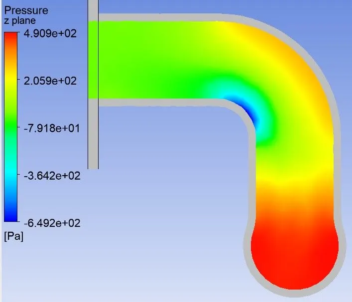
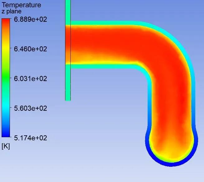
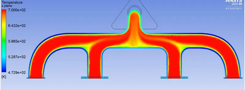
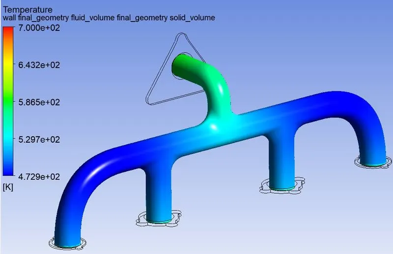
• Create X, Z plane and plot velocity, pressure, temperature & Wall heat transfer coefficient contours on the z plane.
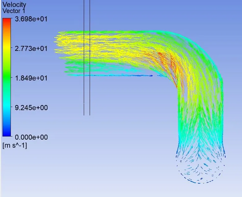
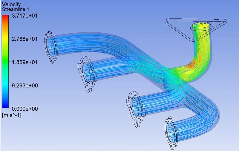
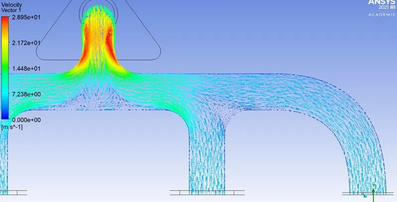
• Create velocity streamline and velocity vectors
• Create velocity vectors and streamlines on the Z plane.

Mass conservation:

index 1,2,3,4 are 4 inlets o is outlet index

`A_1*V_1+A_2*V_2+A_3*V_3+A_4*V_4 = A_o*V_o`

`V_1=V_2=V_3=V_4 = V_i = 5 text( m/s)`

`D_1 =D_2=D=3= D_4 =D_i= 0.16999 text( m)`

`D_o = 0.15 text( m)`

`V_o = (V_i *4*(pi/4)*D_i^2)/((pi/4)*D_o^2)`

`V_o = (5*4*0.16999^2)/0.15^2=25.685`

	Analytical solution from Mass conservation	Numerical solution from simulation	Error
Outlet Velocity	25.685	25.19	0.0192

Problem Definition

Hot air at 700K is flowing through the Exhaust manifold with a velocity of 5 m/s which is made up of Aluminium material. open Air outside manifold at 300K with Heat transfer coefficient = 20 W/m^2-K.

Analytical Solution:

Heat Transfer in exhaust manifold done in 3 stages firstly heat being convected forcefully from Hot air to pipe internal surface after that convected heat is getting conducted through the solid pipe wall and reaches pipe external surface. Finally, this conducted heat is convected to the outer atmosphere naturally because the solid body and the surrounding air is at standstill condition.

How would you verify if the HTC predictions from the simulations are right

We use following emperical relation to validate Heat transfer co-efficient predictions from simulation they are:

Dittus-Boelter heat transfer coefficient correlation to calculate the nusselt number.

`text(Nusselt Number = )N_u = 0.023*R_(e)^0.8*P_r^n`

Validity:

`0.6<=P_r<=160`

`Re_(Dh)>10000`

`L/D = 10`

`text(Renoulds number = ) R_e = (rho*V*D)/mu`

`text(Prandtl number = ) P_r = (mu*C_p)/k`

We also that Nusselt Number `N_u = (h*l)/k`

`h = (N_u*k)/l`

`h = text(Heat transfer coefficient W/m^2-K)`

`rho = text(Density kg/m^3)`

`V = text(Velocity m/s)`

`D = text(Diameter m)`

`mu = text(Dynamic Viscosity kg/m-s)`

`C_p = text(specific Heat of Fluid j/kg-K)`

`k = text(Thermal conductivity of fluid W/m⋅K)`

`text(For Cooling )n = 0.3`

`text(For Heating )n = 0.4`

`L = text(characteristic length D in m)`

Finally, `h text( )alpha text( ) N_u text( ) alpha text( ) R_e text( ) alpha text( )V`

Heat transfer coefficient is proportional to Nusselt number, Nusselt number is proportional to Renolds number which is directly proportional to flow Velocity.

On what factors does the accuracy of the prediction depend on?

• In Heat Transfer simulations accuracy mainly depend on the size and number of inflation layers according to the Viscous model chosen.
• Another main factor is Mesh Refinement & Element size.