Week 4 - Genetic Algorithm

Optimization of the Stalagmite Function using Genetic Algorithm

Aim: -

Writing a MATLAB program to optimize the stalagmite function and find the Global Maxima of the function.

Objectives: -

1. Able to optimize the stalagmite function and find the global maxima of the function.
2. Able to explain the concept of genetic algorithm & syntax for GA in MATLAB.
3. Plot graphs for F maximum vs no. of iterations for all studies.

Stalagmite theory

A stalagmite is a type of rock formation that rises from the floor of a cave due to the accumulation of material deposited on the floor from ceiling drippings. Stalagmites are typically composed of calcium carbonate but may consist of lava, mud, pear, pitch, sand.

Stalagmite function

`f = f1x.f2x.f1y.f2y`

`f1x = [sin(5.1*pi*x+0.5)]^6`

`f1y = [sin(5.1*pi*y+0.5)]^6`

`f2x = exp[-4ln(2)(x-0.06667)^2/0.64]`

Genetic algorithm

A genetic algorithm is a search heuristic that is inspired by Charles Darwin’s theory of natural evolution. This algorithm reflects the process of natural selection where the fittest individuals are selected for reproduction in order to produce offspring of the next generation.

Five phases are considered in a genetic algorithm.

1. Initial population: - The process begins with a set of individuals which is called a Population. Each individual is a solution to the problem you want to solve.
2. Fitness function: - The fitness function determines how to fit an individual is (the ability of an individual to compete with other individuals). It gives a fitness score to each individual. The probability that an individual will be selected for reproduction is based on its fitness score.
3. Selection: - The idea of the selection phase is to select the fittest individuals and let them pass their genes to the next generation. Two pairs of individuals (parents) are selected based on their fitness scores. Individuals with high fitness have more chances to be selected for reproduction.
4. Crossover: - Crossoveris the most significant phase in a genetic algorithm. For each pair of parents to be mated, a crossover point is chosen at random from within the genes.
5. Mutation: - In certain new offspring formed, some of their genes can be subjected to a mutation with a low random probability. This implies that some of the bits in the bit string can be flipped.

GA syntax

x = ga(fun,nvars)

x = ga(fun,nvars,A,b)

x = ga(fun,nvars,A,b,Aeq,beq)

x = ga(fun,nvars,A,b,Aeq,beq,lb,ub)

x = ga(fun,nvars,A,b,Aeq,beq,lb,ub,nonlcon)

x = ga(fun,nvars,A,b,Aeq,beq,lb,ub,nonlcon,options)

x = ga(fun,nvars,A,b,[],[],lb,ub,nonlcon,IntCon)

x = ga(fun,nvars,A,b,[],[],lb,ub,nonlcon,IntCon,options)

x = ga(problem)

[x,fval] = ga(___)

[x,fval,exitflag,output] = ga(___)

[x,fval,exitflag,output,population,scores] = ga(___)

fitnessfcn	Fitness functions
nvars	Number of design variables
Aineq	A matrix for linear inequality constraints
Bineq	b vector for linear inequality constraints
Aeq	Aeq matrix for linear equality constraints
Beq	beq vector for linear equality constraints
lb	Lower bound on x
ub	Upper bound on x
nonlcon	Nonlinear constraint function
rngstate	Optional field to reset the state of the random number generator
solver	'ga'
options	Options created using optimoptions or an options structure
x	Solution
fval	Objective function value at the solution.
exitflag	Reason that ga stopped.
output	Information about the optimization process
population	Final population
scores	Final scores

Procedure: -

1. Create a function file for the stalagmite function.
2. Create a new script file, define x, y range, and create a mesh grid for xx, yy.
3. Find stalagmite function solutions for xx, yy.
4. Use GA to find optimal solutions.
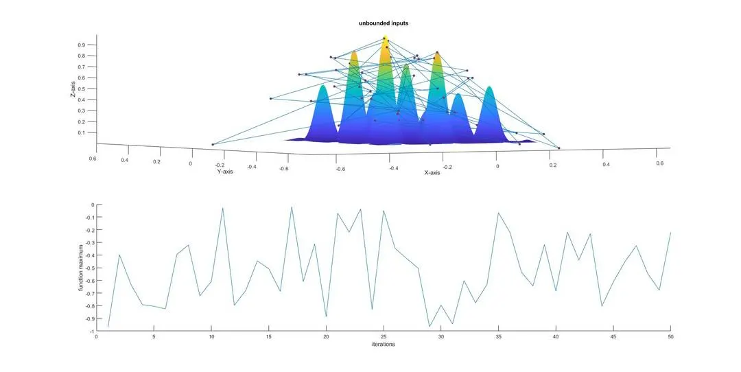
5. Create a loop1 for GA with unbounded inputs and plot the results.
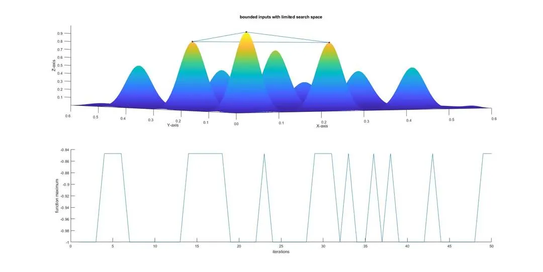
6. Create a loop1 for GA with bounded input search space limit to GA and plot the results.
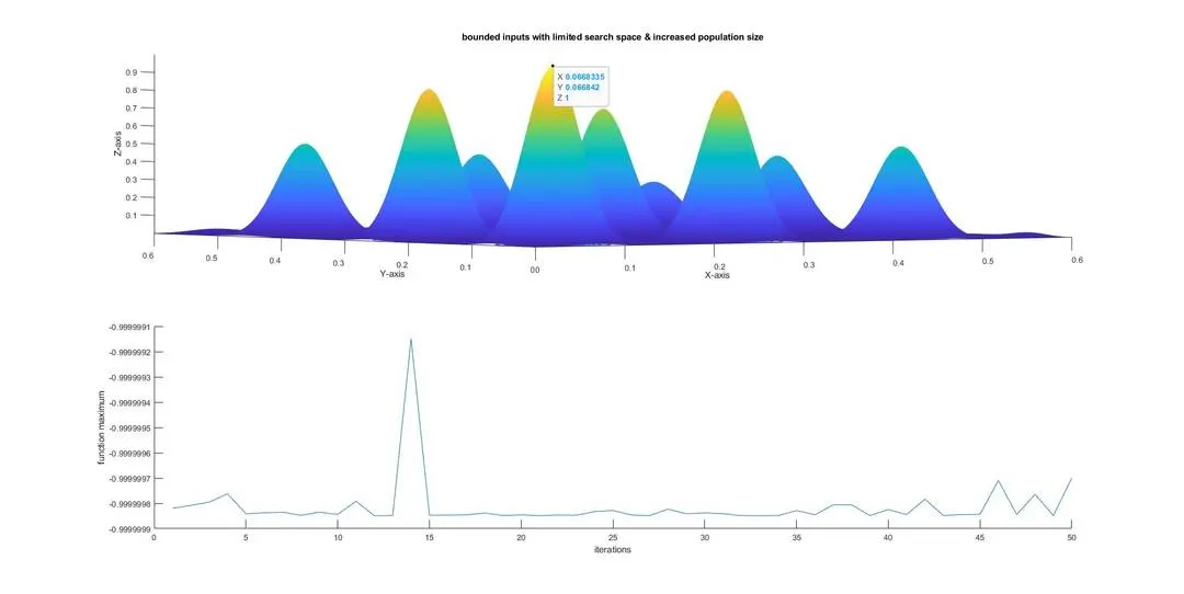
7. Create a loop1 for GA with bounded input search space limit & increased population size to GA and plot the results.

functional code1:-

function  [f]= stalagmite(input_vector); %single input argument stalagmite function to find global maxima
x = input_vector(1); 
y = input_vector(2);
f1x = (sin(5.1*pi*x+0.5))^6;
f2x = exp(-4*log(2)*(((x-0.0667)^2)/0.64));
f1y = (sin(5.1*pi*y+0.5))^6;
f2y = exp(-4*log(2)*(((y-0.0667)^2)/0.64));
f = -(f1x*f2x*f1y*f2y); 
%actually there is no '-' sign for stalagmite function but we introduced - sign because we are going to use GA to find maxima. actually GA will
%predict minimum value. if we multifly - to function maximum value become minimum, mimimum become maximum 
end

functional code2:-

function  [f]= get_stalagmite(x,y);
f1x = (sin(5.1*pi*x+0.5)).^6;
f2x = exp(-4*log(2)*(((x-0.0667).^2)/0.64));
f1y = (sin(5.1*pi*y+0.5)).^6;
f2y = exp(-4*log(2)*(((y-0.0667).^2)/0.64));
f = f1x.*f2x.*f1y.*f2y;
end

Main code:-

clear all; close all; clc

x = linspace(0,0.6,150);                                                 %x range & divisions
y = linspace(0,0.6,150);                                                 %y range & divisions
[xx, yy] = meshgrid(x,y);                                                   %creating 2-D mesh with x,y
num_cases = 50;                                                             %number of iterations to solve
f = get_stalagmite(xx,yy);                                                  %solve the get_stalagmite function and assign the values to f
%------------------------------------------------------------------------------------------------------------------
%study 1 --statistical behaviour for un bounded inputs
tic                                                                         %timer starts          
for i = 1:num_cases                                                         %iterations loop start
  [inputs1,foptimum1(i)] = ga(@stalagmite,2);                               %solving GA for stalagmite function for 2variables
  xoptimum1(i) = inputs1(1);
  yoptimum1(i) = inputs1(2);
end
stydy_time_1 = toc;                                                         %timer stop
figure(1)                                                                   %ploting results
subplot(2,1,1); 
hold on;
surfc(xx,yy,f);                                                             %creating surface of stalagmite function
xlabel('X-axis');   ylabel('Y-axis');   zlabel('Z-axis');   shading interp; % labeling and shading
plot3(xoptimum1,yoptimum1,-foptimum1,'marker','o','markersize',4,'markerfacecolor','r'); %plotting GA points
title('unbounded inputs');
subplot(2,1,2);
hold on;
plot(foptimum1);                                                             %ploting optimum values for each iteration
xlabel('iterations');   ylabel('function maximum');
%---------------------------------------------------------------------------------------------------------------
%study 2 -- statistical behaviour for bounded input search space limit to GA
tic
for i = 1:num_cases
  [inputs2,foptimum2(i)] = ga(@stalagmite,2,[],[],[],[],[0,0],[0.6,0.6]);%defining search space range [0,0],[0.6,0.6]
  xoptimum2(i) = inputs2(1);
  yoptimum2(i) = inputs2(2);
end
stydy_time_2 = toc;
figure(2)
subplot(2,1,1) ;
hold on;
surfc(xx,yy,f);
xlabel('X-axis');   ylabel('Y-axis');  zlabel('Z-axis');    shading interp;
plot3(xoptimum2,yoptimum2,-foptimum2,'marker','o','markersize',4,'markerfacecolor','r');
title('bounded inputs with limited search space');
subplot(2,1,2);
hold on;
plot(foptimum2); 
xlabel('iterations');   ylabel('function maximum');
%------------------------------------------------------------------------------------------------------------------
%study 3 -- statistical behaviour bounded input search space limit & increased population size  to GA
options = optimoptions('ga','populationsize',200);                           %optimooptions used to add population size to GA
tic
for i = 1:num_cases
  [inputs3,foptimum3(i)] = ga(@stalagmite,2,[],[],[],[],[0,0],[0.6,0.6],[],[],options); %adding populationsize through options
  xoptimum3(i) = inputs3(1);
  yoptimum3(i) = inputs3(2);
end
stydy_time_3 = toc;
figure(3)
subplot(2,1,1) ;
hold on;
surfc(xx,yy,f);
xlabel('X-axis');   ylabel('Y-axis');   zlabel('Z-axis');   shading interp;
plot3(xoptimum3,yoptimum3,-foptimum3,'marker','o','markersize',4,'markerfacecolor','r');
title('bounded inputs with limited search space & increased population size');
subplot(2,1,2);
hold on;
plot(foptimum3);
xlabel('iterations');   ylabel('function maximum');

Graphs:-