Project 2 - Rankine cycle Simulator
Rankine Cycle Simulator
Aim: -
To create a Rankine Cycle Simulator using MATLAB.
Objectives: -
- Able to calculate the state points of the Rankine Cycle based on user inputs.
- Able to plot T-s and h-s graphs for the given inputs.
Description: -
The Rankine cycle is a model used to predict the performance of steam turbine systems. It was also used to study the performance of reciprocating steam engines. The Rankine cycle is an idealized thermodynamic cycle of a heat engine that converts heat into mechanical work while undergoing phase change. It is an idealized cycle in which friction losses in each of the four components are neglected. The heat is supplied externally to a closed loop, which usually uses water as the working fluid.
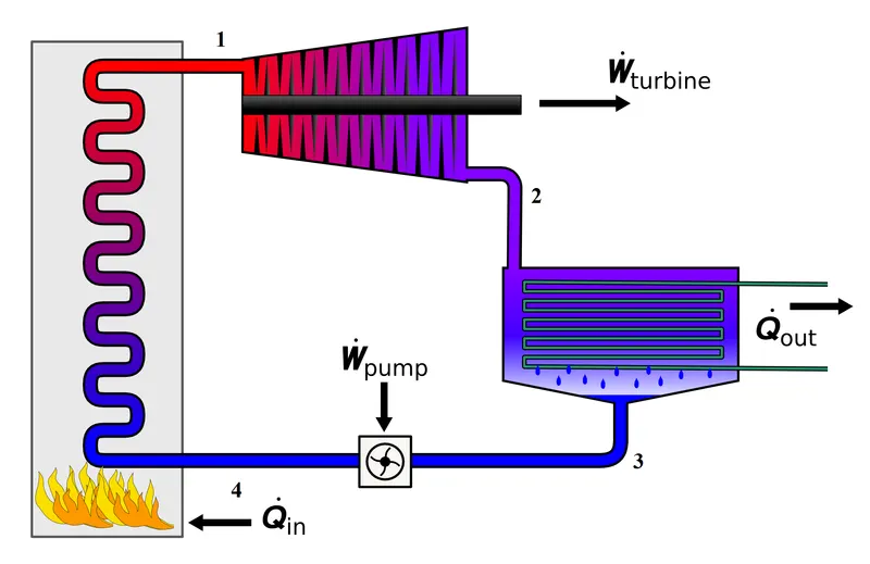
1-2 is Isentropic Expansion in the Turbine
2-3 is constant Pressure Heat Rejection by the Condenser
3-4 is Isentropic Compression in the Pump
4-1 is constant Pressure Heat Addition by the Boiler
- Enthalpy, H: - the sum of the internal energy and the product of the pressure and volume of a thermodynamic system.
- Entropy, S: - the measure of a system's thermal energy per unit temperature that is unavailable for doing useful work.
- Back-work ratio: - The ratio of the pump work to the turbine work is called the back-work ratio
Formulae: -
Liquid state: -
`H = Cp.dt`
`S = Cp.ln((T1) /(T2))`
Liquid & Vapour state: -
`H = hf + x.(hg-hf)`
`S = Sf + x.(Sg-Sf)`
Vapor state: -
`H = hg + m.Cp.dt`
`S =Sg+ Cp.ln((T1) /(T2))`
f represents the respective h, s value at saturated liquid state.
g represents the respective h, s value at saturated vapour state.
x = dryness fraction.
`text(Turbine work) = h1-h2`
`text(Pump work) = h4-h3`
`text(Net work) = text(Turine work)-text(Pump work)`
`text(Heat supplied) = h1-h4`
`text(Heat rejected) = h2-h3`
`text(Efficiency) =text(Net work)/text(Heat supplied)`
`text(Back work ratio) = text(Pump work)/text(Turbine work)`
Procedure: -
- Take inputs for Turbine Inlet, outlet Pressure (in bars), Turbine inlet Temperature (in Degree Celsius).
- Extract data for H, S from XStream library using input variables.
- Find state point one using input data.
- 1-2 is Isentropic Expansion in the Turbine, to find state variables at point 2 equate entropy at both state points are equal.
- Find x dryness value at point 2 if it is greater than 1 then point 2 lies in the super-heated region else it lies in the liquid vapour region.
- 2-3 is constant Pressure Heat Rejection by the Condenser in this process pressure and the temperature remains constant due to phase change. Point 3 will lie on the liquidus line.
- 3-4 is Isentropic Compression in the Pump To find state variables at point 4 equate entropy at both state points are equal.
- Calculate the turbine work, compressor work, net-work, Back Work Ratio, thermal efficiency, specific steam consumption.
- Plot T-S, H-S diagrams
Main Program: -
clear all; close all; clc;

A = '        RANKINE CYCLE SIMULATOR';                        disp(A)
B = '1-2 is Isentropic Expansion in the Turbine';             disp(B)
C = '2-3 is const Pressure Heat Rejection by the Condenser';  disp(C)
D = '3-4 is Isentropic Compression in the Pump';              disp(D)
E = '4-1 is const Pressure Heat Addition by the Boiler';      disp(E)
%%
P_T   = 'Turbine Inlet Pressure (in bar): ';
T_T1  = 'Turbine intet Temperature (in Degree Celsius): ';
P_C   = 'Turbine outlet (or) Condenser Inlet Pressure (in bar) : ';

 P1 = str2double(string(inputdlg(P_T)));
 P2 = str2double(string(inputdlg(P_C)));
 T1 = str2double(string(inputdlg(T_T1)));

disp('------------------------------------------------------')
% C1 = sprintf('%s %.4f',P_T,string(P1));                 disp(C1);
% C2 = sprintf('%s %.4f',T_T1,string(T1));                disp(C2);
% C3 = sprintf('%s %.4f',P_C,string(P2));                 disp(C3);

C1 = sprintf('%s %.4f',P_T,P1);                 disp(C1);
C2 = sprintf('%s %.4f',T_T1,T1);                disp(C2);
C3 = sprintf('%s %.4f',P_C,P2);                 disp(C3);

%%
%%
%high pressure P1 conditions
Tsat_1 = XSteam('Tsat_p',P1);
Hf_1   = XSteam('hL_p',P1);
Hg_1   = XSteam('hV_p',P1);
Hfg_1  = Hg_1-Hf_1;
Sf_1   = XSteam('sL_p',P1);
Sg_1   = XSteam('sV_p',P1);
Sfg_1  = Sg_1-Sf_1;
Vf_1   = XSteam('vL_p',P1);
Vg_1   = XSteam('vV_p',P1);
Cp_L_1 = XSteam('CpL_p',P1);
CP_V_1 = XSteam('CpV_p',P1);
%%
%%
%low pressure P2 conditions
Tsat_2 = XSteam('Tsat_p',P2);
Hf_2   = XSteam('hL_p',P2);
Hg_2   = XSteam('hV_p',P2);
Hfg_2  = Hg_2-Hf_2;
Sf_2   = XSteam('sL_p',P2);
Sg_2   = XSteam('sV_p',P2);
Sfg_2  = Sg_2-Sf_2;
Vf_2   = XSteam('vL_p',P2);
Vg_2   = XSteam('vV_p',P2);
Cp_L_2 = XSteam('CpL_p',P2);
CP_V_2 = XSteam('CpV_p',P2);
 %%
%% At state point 1:
disp('------------------------------------------------------')
disp('At state point 1:')
if T1 > Tsat_1
    disp('Superheated steam is entering in to the turbine')
elseif T1 == Tsat_1
     disp('Saturated steam is entering in to the turbine')
else, T1 < Tsat_1;
    disp('Stop the Unit')
    disp('Steam with water molecules are entering in to the turbine it may damage the turbine blades')
end
S1  = XSteam('s_pT',P1,T1);
H1  = XSteam('h_pT',P1,T1);
s_p1 = sprintf('Pressure    P1  = %5.5f bar',P1);         disp(s_p1);
s_t1 = sprintf('Temperature T1  = %5.5f Deg Celsius',T1); disp(s_t1);
s_h1 = sprintf('Enthalpy    H1  = %5.5f kj/kg',H1);       disp(s_h1);
s_s1 = sprintf('Entropy     S1  = %5.5f kj/kgK',S1);      disp(s_s1);
%%
%% At state point 2:
disp('------------------------------------------------------')
disp('At state point 2:')
S2 = S1;
x = ((S1-Sf_2)/Sfg_2);
if (x > 0) && (x <= 1)
    H2 = Hf_2 + (x*Hfg_2);
    T2 = Tsat_2;
elseif x > 1
    T2 = (exp((S1-Sg_2)/CP_V_2)) * Tsat_2;
    H2 = Hg_2 + (CP_V_2*(T2-Tsat_2)) ;
    disp('Turbine outlet steam is, still in Super heated form (energy going as waste)')
end
s_p2 = sprintf('Pressure    P2  = %5.5f bar',P2);         disp(s_p2);
s_t2 = sprintf('Temperature T2  = %5.5f Deg Celsius',T2); disp(s_t2);
s_h2 = sprintf('Enthalpy    H2  = %5.5f kj/kg',H2);       disp(s_h2);
s_s2 = sprintf('Entropy     S2  = %5.5f kj/kgK',S2);      disp(s_s2);
%%
%% At state point 3:
disp('------------------------------------------------------')
disp('At state point 3:')
P3  = P2;
T3  = Tsat_2;                %during phase temperature remains constant
H3  = Hf_2;
S3  = Sf_2;
V3  = Vf_2;
s_p3 = sprintf('Pressure    P3  = %5.5f bar',P3);         disp(s_p3);
s_t3 = sprintf('Temperature T3  = %5.5f Deg Celsius',T3); disp(s_t3);
s_h3 = sprintf('Enthalpy    H3  = %5.5f kj/kg',H3);       disp(s_h3);
s_s3 = sprintf('Entropy     S3  = %5.5f kj/kgK',S3);      disp(s_s3);
%%
%%
% At state point 4:
disp('------------------------------------------------------')
disp('At state point 4:')
P4  = P1;
S4  = S3;
T4  = Tsat_1/(exp((Sf_1-S3)/Cp_L_1));
P_w = Vf_2 * (P4-P3) * 100;
H4  = H3 + P_w;
s_p4 = sprintf('Pressure    P4  = %5.5f bar',P4);         disp(s_p4);
s_t4 = sprintf('Temperature T4  = %5.5f Deg Celsius',T4); disp(s_t4);
s_h4 = sprintf('Enthalpy    H4  = %5.5f kj/kg',H4);       disp(s_h4);
s_s4 = sprintf('Entropy     S4  = %5.5f kj/kgK',S4);      disp(s_s4);
%%
%%
disp('------------------------------------------------------')
%1-2 is Isentropic Expansion in the Turbine work done by Turbine
W_T = H1-H2;
%2-3 is const Pressure Heat Rejection by the Condenser
Q_R = H2-H3;
%3-4 is Isentropic Compression in the Pump work supplied to pump
W_P = P_w;
%4-1 is const Pressure Heat Addition by the Boiler
Q_S = H1-H4;
%%
% Net work
W_N = W_T-W_P;
% Efficiency
eff = (W_N/Q_S)*100;
SSC = 3600/W_T;
BWR  = W_P/W_T;
%%
Turbine_work = sprintf('Turbine_work         = %5.5f kj/kg',W_T);           disp(Turbine_work)
Pump_work    = sprintf('Pump_work            = %5.5f kj/kg',W_P);           disp(Pump_work)
Net_work     = sprintf('Net_work             = %5.5f kj/kg',W_N);           disp(Net_work)
Thermal_effi = sprintf('Thermal_efficiency   = %5.5f',eff);                 disp(Thermal_effi)
S.S.C        = sprintf('Specific Steam Consumption = %5.5f kg/kwh',SSC);    disp(S.S.C)
back_work     = sprintf('Back Work Ratio     = %5.5f kj/kg',BWR);           disp(back_work)
%%
%%
T = linspace(1,373.9,150);  %373.9 deg celcius is the critical temperature of water
for i = 1:length(T)
    SL(i) = XSteam('sL_T',T(i));
    SV(i) = XSteam('sV_T',T(i));
    HL(i) = XSteam('hL_T',T(i));
    HV(i) = XSteam('hV_T',T(i));
end
%%
%plotting 1 T-S diagram
figure(1); hold on
plot([S1, S2],[T1, T2],'r','linewidth',2);             text(S1,T1,'  1');
%'DisplayName','1-2 is Isentropic Expansion in the Turbine',
if T2 == Tsat_2
    plot([S2, S3],[T2, T3],'r','linewidth',2);         text(S2,T2,'  2');
else
    plot([S2, Sg_2],[T2, Tsat_2],'r','linewidth',2);   text(S2,T2,'  2');
    plot([Sg_2, S3],[Tsat_2, T3],'r','linewidth',2);   text(Sg_2,Tsat_2,'  2^');
end
plot([S3, S4],[T3, T4],'r','linewidth',2);             text(S3,T3,'  3');
plot([S4, Sf_1],[T4, Tsat_1],'r','linewidth',2);       text(S4,T4,'  4');
plot([Sf_1, Sg_1],[Tsat_1, Tsat_1],'r','linewidth',2); text(Sf_1,Tsat_1,'  4^');
plot([Sg_1, S1],[Tsat_1, T1],'r','linewidth',2);       text(Sg_1,Tsat_1,'  1^');
plot(SL,T,'b--');
plot(SV,T,'b--');
xlabel('(S)Entropy kj/kgK');  ylabel('(T)Temperature (Deg Celsius)'); title('RANKINE CYCLE T-S diagram'); grid on;
saveas(1,'T-S diagram.jpg')
%%
%plotting 2 H-S diagram
figure(2); hold on
plot([S1, S2],[H1, H2],'r','linewidth',2);             text(S1,H1,'  1');
if T2 == Tsat_2
    plot([S2, S3],[H2, H3],'r','linewidth',2);         text(S2,H2,'  2');
else
    plot([S2, Sg_2],[H2, Hg_2],'r','linewidth',2);     text(S2,H2,'  2');
    plot([Sg_2, S3],[Hg_2, H3],'r','linewidth',2);     text(Sg_2,Hg_2,'  2^');
end
plot([S3, S4],[H3, H4],'r','linewidth',2);             text(S3,H3,'  3');
plot([S4, Sf_1],[H4, Hf_1],'r','linewidth',2);         text(S4,H4,'  4');
plot([Sf_1, Sg_1],[Hf_1, Hg_1],'r','linewidth',2);     text(Sf_1,Hf_1,'  4^');
plot([Sg_1, S1],[Hg_1, H1],'r','linewidth',2);         text(Sg_1,Hg_1,'  1^');
plot(SL,HL,'b--')
plot(SV,HV,'b--')
xlabel('(S)Entropy kj/kgK');  ylabel('(H)Enthalpy kj/kg'); title('RANKINE CYCLE H-S diagram'); grid on;
saveas(2,'H-S diagram.jpg')
%%
Results: -
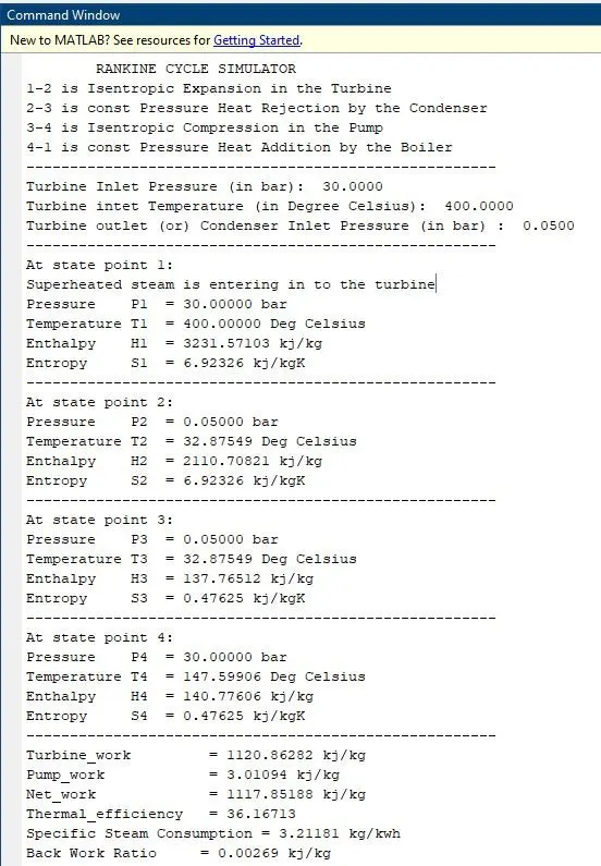
Graphs:-
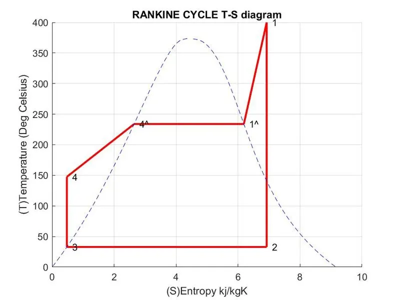
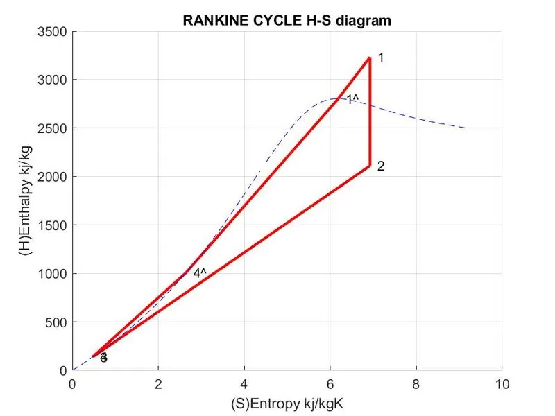
1-2 is Isentropic Expansion in the Turbine.
2-3 is const Pressure Heat Rejection by the Condenser.
3-4 is Isentropic Compression in the Pump.
4-1 is const Pressure Heat Addition by the Boiler.
4^ point represents the starting of fluid phase change from liquid to vapour.
If the turbine outlet fluid is still in super heated state then expected graphs as follows:-

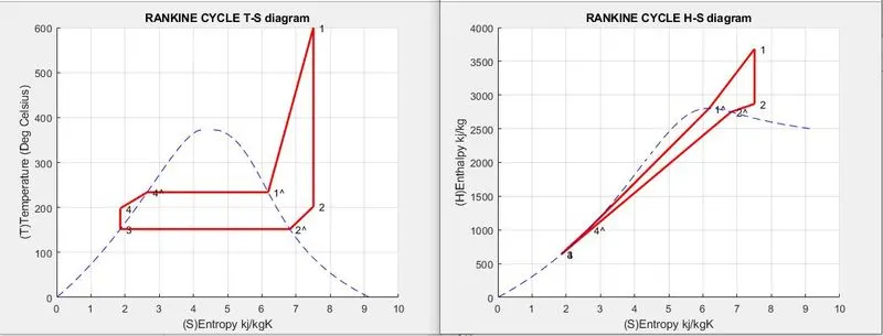
2^^ point represents the starting of Vapour phase change from vapour to liquid.
References:-
https://en.wikipedia.org/wiki/Rankine_cycle
https://in.mathworks.com/help/matlab/ref/inputdlg.html
https://in.mathworks.com/help/matlab/ref/sprintf.html
https://in.mathworks.com/help/matlab/ref/disp.html
https://in.mathworks.com/help/matlab/ref/if.html