Week 3 - Taylor table method and Matlab code

Taylor table method to solve 4th order approximations of the second-order derivative

Aim: -

To write a program that compares the Central, Skewed right-sided & Skewed left-sided difference 4th order approximations for second-order derivative. against the analytical or exact derivative for a range dx of function f(x) = exp(x)*cos(x) .

Objectives: -

1. Able to compute the 2nd derivative 4th order approximations of function f(x) = exp(x)*cos(x) at x = pi/3 for dx range = [pi/4000,pi/40,20] for Central, Skewed right-sided & Skewed left-sided schemes
2. Find error parameter as the absolute difference in numerical and exact derivative at x = pi/3 for all schemes.
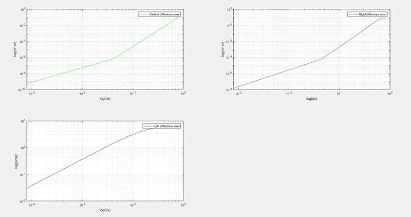
3. Plot the errors vs dx

Schemes to solve approximations

1. Central/ symmetric difference scheme
2. Skewed right-sided difference scheme
3. Skewed left-sided difference scheme

The order of accuracy P = Number of nodes in the stencil N - order of derivative Q + 1 for symmetric/central schemes

The order of accuracy P = Number of nodes in the stencil N - order of derivative Q for one-sided/skewed schemes

Description: -

function `f(x) = exp(x)*cos(x)`

analytical/exact derivative of `f''(x) = -2*exp(x)*sin(x)`

numerical derivative using tailors table for 4th order approximations of the second-order derivative

`text(Central difference) =(a*exp(x-2*dx)*cos(x-2*dx)+b*exp(x-dx)*cos(x-dx)+c*exp(x)*cos(x)+d*exp(x+dx)*cos(x+dx)+e*exp(x+2*dx) *cos(x+2*dx))/dx^2`

`text(Right difference) =(a*exp(x)*cos(x)+b*exp(x+dx)*cos(x+dx)+c*exp(x+2*dx)*cos(x+2*dx)+d*exp(x+3*dx)*cos(x+3*dx)+e*exp(x+4*dx)*cos(x+4*dx)+f*exp(x+5*dx)*cos(x+5*dx))/(dx^2)`

`text(Left difference) =(a*exp(x)*cos(x)+b*exp(x-dx)*cos(x-dx)+c*exp(x-2*dx)*cos(x-2*dx)+d*exp(x-3*dx)*cos(x-3*dx)+e*exp(x-4*dx)*cos(x-4*dx)+f*exp(x-5*dx)*cos(x-5*dx))/(dx^2)`

`text(Error = numerical derivative - analytical derivative)`

Procedure: -

1. function program
2. create tailor matrix.
3. find the number nodes required for various schemes, based on number of nodes extract proper matrix from tailor table.
4. find constants, by using constants, & inputs x ,dx find Central, Skewed right-sided & Skewed left-sided difference
5. Main Program
6. find analytical derivative.
7. Using the above function find Central, Skewed right-sided & Skewed left-sided difference and subtract analytical derivative from to get error
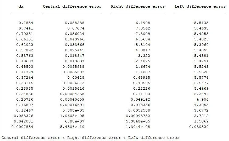
8. Tabulate the errors.
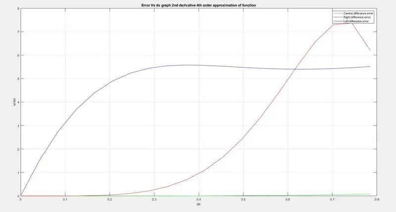
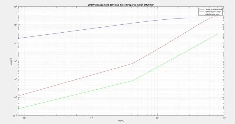
9. Plot the normal & log-log graphs for errors.
10. find the slope of the curves generated.

function code for 4th order approximations of the second-order derivative: -

function [central_diff, right_diff, left_diff] = approx_4th_order_2nd_derivative(x,dx)

%tailor matrix for second order derivative
tailor_matrix1 = [
    1 1 1 1 1 1 1 1 1 1 1;
    -5 -4 -3 -2 -1 0 1 2 3 4 5;
    25/2 16/2 9/2 4/2 1/2 0 1/2 4/2 9/2 16/2 25/2;
    -125/6 -64/6 -27/6 -8/6 -1/6 0 1/6 8/6 27/6 64/6 125/6;
    625/24 256/24 81/24 16/24 1/24 0 1/24 16/24 81/24 256/24 625/24;
    -3125/120 -1024/120 -243/120 -32/120 -1/120 0 1/120 32/120 243/120 1024/120 3125/120];
% a = accuracy;
% o = order;
% central_nodes = a + o - 1 = 4 + 2 - 1 = 5
% one_side_nodes = a + o = 4 + 2 = 6

%Central difference tailor matrix
central = tailor_matrix1(1:5,4:8);
%Skewed right-sided difference tailor matrix
right   = tailor_matrix1(1:6,6:11);
% Skewed left-sided difference difference tailor matrix
left    = tailor_matrix1(1:6,1:6);

%for second order derivative
A = [0; 0; 1; 0; 0];
B = [0; 0; 1; 0; 0; 0];
%
central_coeff = central\A;
right_coeff = right\B;
left_coeff = left\B;

c = central_coeff;
r = right_coeff;
l = left_coeff;

%1. Central difference
central_diff = (c(1)*exp(x-2*dx)*cos(x-2*dx)+c(2)*exp(x-dx)*cos(x-dx)+c(3)*exp(x)*cos(x)+c(4)*exp(x+dx)*cos(x+dx)+c(5)*exp(x+2*dx) *cos(x+2*dx))/dx^2;
%2. Skewed right-sided difference
right_diff   = (r(1)*exp(x)*cos(x)+r(2)*exp(x+dx)*cos(x+dx)+r(3)*exp(x+2*dx)*cos(x+2*dx)+r(4)*exp(x+3*dx)*cos(x+3*dx)+r(5)*exp(x+4*dx)*cos(x+4*dx)+r(6)*exp(x+5*dx)*cos(x+5*dx))/dx^2;
%3. Skewed left-sided difference
left_diff    = (l(1)*exp(x)*cos(x)+l(2)*exp(x-dx)*cos(x-dx)+l(3)*exp(x-2*dx)*cos(x-2*dx)+l(4)*exp(x-3*dx)*cos(x-3*dx)+l(5)*exp(x-4*dx)*cos(x-4*dx)+l(6)*exp(x-5*dx)*cos(x-5*dx))/dx^2;

end

Main program: -

clear all; close all; clc;

x = pi/3;
dx = linspace(pi/4,pi/4000,20);
% analytical function f(x) = e^x*cos(x);
% analytical derivative f'(x) = e^x*cos(x)-e^x*sin(x); f''(x) = -2e^x*sin(x)

analytical_derivative = -2*exp(x)*sin(x);

for i = 1:length(dx)
    [Central_diff(i), Right_diff(i), Left_diff(i)] = approx_4th_order_2nd_derivative(x,dx(i));
    Central_diff_error(i) = abs(Central_diff(i)-analytical_derivative);
    Right_diff_error(i) = abs(Right_diff(i)-analytical_derivative);
    Left_diff_error(i) = abs(Left_diff(i)-analytical_derivative);
end
error_table = table(dx',Central_diff_error',Right_diff_error',Left_diff_error','VariableName',{'dx','Central difference error','Right difference error','Left difference error'})
disp('Central difference error < Right difference error < Left difference error')

figure(1);
plot(dx,Central_diff_error,'g')
hold on
plot(dx,Right_diff_error,'r')
plot(dx,Left_diff_error,'b')
xlabel('dx'); ylabel('error'); grid on
legend('Central difference error','Right difference error','Left difference error')
title('Error Vs dx graph 2nd derivative 4th order approximation of function')

figure(2); 
loglog(dx,Central_diff_error,'g')
 hold on
loglog(dx,Right_diff_error,'r')
loglog(dx,Left_diff_error,'b')
xlabel('log(dx)'); ylabel('log(error)'); grid on
legend('Central difference error','Right difference error','Left difference error')
title('Error Vs dx graph 2nd derivative 4th order approximation of function')

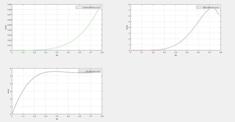
figure(3);  
subplot(2,2,1)
plot(dx,Central_diff_error,'g')
xlabel('dx'); ylabel('error'); grid on ;legend('Central difference error')
subplot(2,2,2)
plot(dx,Right_diff_error,'r')
xlabel('dx'); ylabel('error'); grid on ;legend('Right difference error')
subplot(2,2,3)
plot(dx,Left_diff_error,'b')
xlabel('dx'); ylabel('error'); grid on ;legend('Left difference error')

figure(4);  
subplot(2,2,1)
loglog(dx,Central_diff_error,'g')
xlabel('log(dx)'); ylabel('log(error)'); grid on ;legend('Central difference error')
subplot(2,2,2)
loglog(dx,Right_diff_error,'r')
xlabel('log(dx)'); ylabel('log(error)'); grid on ;legend('Right difference error')
subplot(2,2,3)
loglog(dx,Left_diff_error,'b')
xlabel('log(dx)'); ylabel('log(error)'); grid on ;legend('Left difference error')

Graphs:-

Result Table:-