Week 4 - CHT Analysis on Exhaust port

AIM: Conjugate heat transfer analysis on exhaust port .

1. Brief description of why and where a CHT analysis is used.
2. Maintainning the y+ value according to the turbulence model and justify the results.
3. Calculate the wall/surface heat transfer coefficient on the internal solid surface & show the velocity & temperature contours in appropriate areas.
4. Verify if the HTC predictions from the simulations are right and what factors does the accuracy of the prediction depend on?

INTRODUCTION

• Conjugate heat transfer simulations are referred to coupled fluid-solid temperature calculations.
• The bundary between the two zones is always a wall and a shadow zone is created automatically by fluent.
• Conjugate heat transfer involves heat exchange that occurs simultaneously by convection a fluid and a adjacent wall and by conduction through the solid.
• As the heat transfer inside the body is governed by the ellipticallaplace equation (or) by prabolic differential equation, while the heat transfer inside the fluid is governed by the elliptical N-S equation (or) parabolic boundary layer equation. The solution of such problems gives the temp. and heat flux distribution on the interface.
• Here the HTC can be calculated by using these results.

examples of conjugate heat transfer :

• Transient heat transfer from a hot plate to flowing fluid on it .
• Study of subsonic-supersonic flows requires conjugation because sub-sonic flows is governed by elliptic (or) parabolic differential equation, while the super-sonic flow is governed by hyperbolic differential equation.
• Heat exchangers

SOLVING AND MODELLING APPROACH

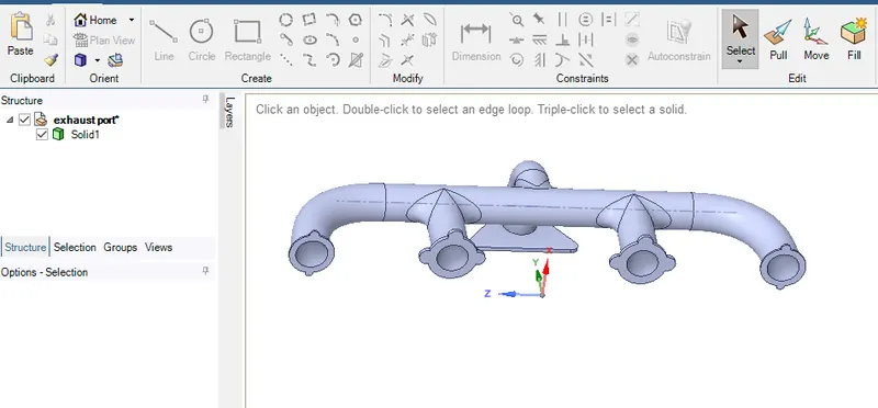
Fig. 1 Exhaust port Geometry

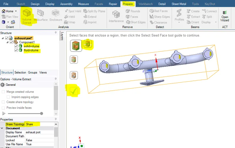
Fig. 2 Volume extraction and creating new component

• The fluid volume is extracted by using extract volume in prepare tab. Then make solid and fluid volume as two differrent entity and assign it to new component under exhaust port as shown above.

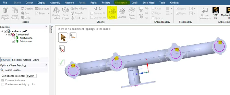
Fig. 3 Share prep

• Share prep is used to connect the outer and inner boundary boundary closed edges where the information can be shared. It is shown in light pink in colour in the fig.

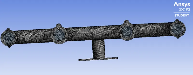
Fig. 4 conformal mesh

• For conjugate heat transfer ,we need body fitted mesh near the boundary or wall. So,far as conduction and convection is considered the mesh near these region needs to be refined to capture the heat transfer coefficient.

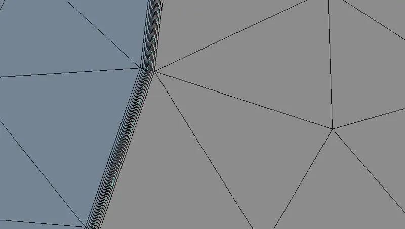
Fig. 5 Inflation layer shown using Y-plus 5

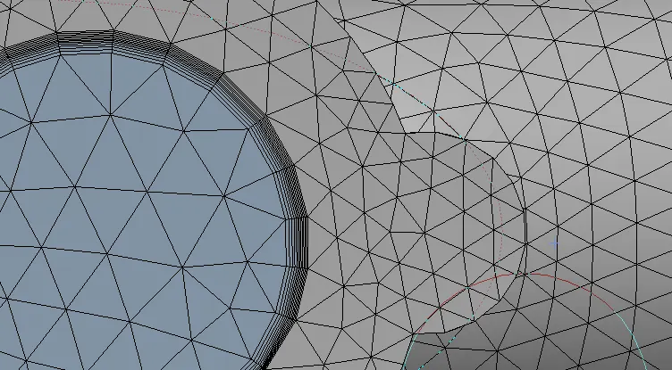
Fig. 6 mesh inflation at Yplus 10

PRE-PROCESSING AND SOLVER SETTING

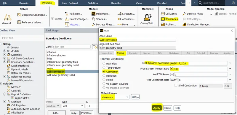
Fig. 7 setting up physics

• The wall boundary is having heat transfer coefficient 20 (w/m2k). The value is for outer surface as the heat is being transfered from the wall to the free stream fluid.

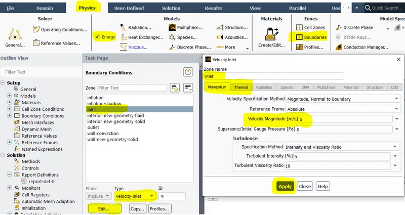
Fig. 8 Definining Boundary condition

• The inlet velocity is given as 5m/s and incoming exhaust fluid temperature is taken as 700K.

Fig. 9 setting up post -processing velocity contour

• Material properties

exhaust manifold =Aluminium

exhaust fluid =Air

Density =1.225kg/m^3

specific heat at const. pressure (Cp) = 1.006 kJ/(kg.K)

Thermal conductivity of free stream (air) =0.024 w/mk at 300k

aluminium thermal conductivity =202.4w/mk

sp.heat Al. = 871 (J/kg.K)

• Boundary Condition

Inlet Air velocity = 5 m/s

Inlet air temperature = 700K

outlet pressure = 0 Pa

Outer exhaust manifold = wall convection

wall heat transfer coefficient = 20 w/m.k

RESULTS

CASE 1

Turbulence model: k-epsilon

element size= 100mm

max. element size = 150mm

Y-plus=30

no. of elements =262428

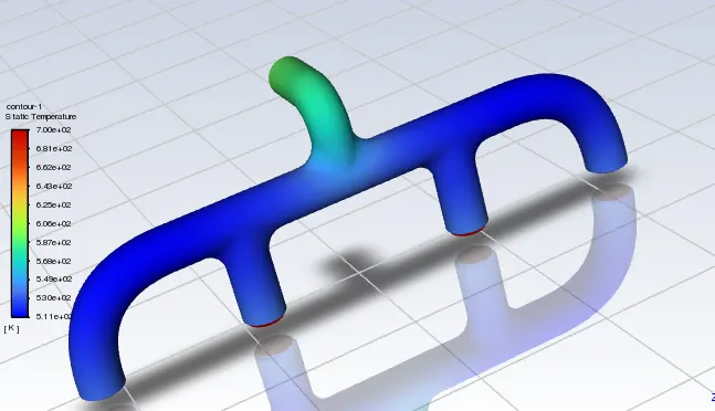
Fig. 10 Temperature animation

• The temperature distribution in the exhaust manifold shown above infers that, there is turbulent mixing of incoming exhaust gases from the exhaust port .
• As there is 4 inlet and 1 exhaust, so the velocity increases to a prominent value.

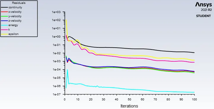
Fig. 11 Residual Vs iteration

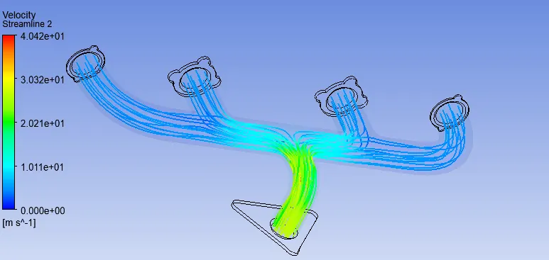
Fig. 12 Velocity streamline

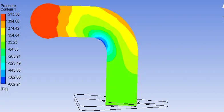
Fig. 13 Plane showing the pressure contour ( region shows negative pressue where velocity increases)

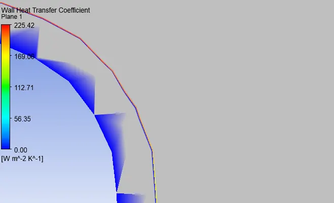
Fig. 14 Wall heat transfer coefficient

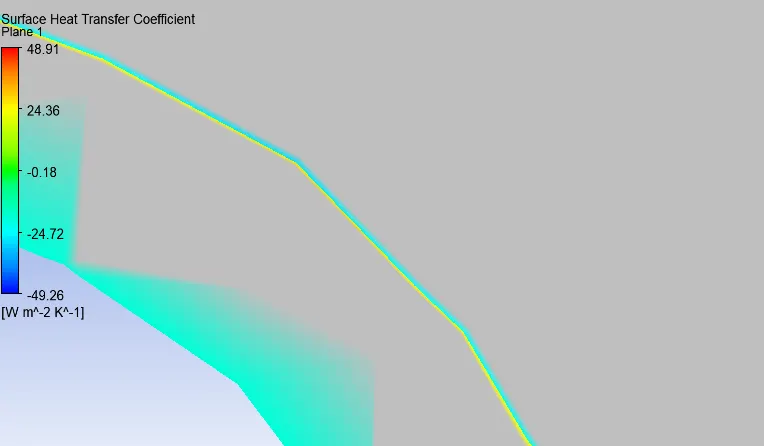
Fig. 15 Surface heat transfer coefficient

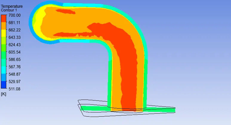
Fig. 16 Temperature Contour

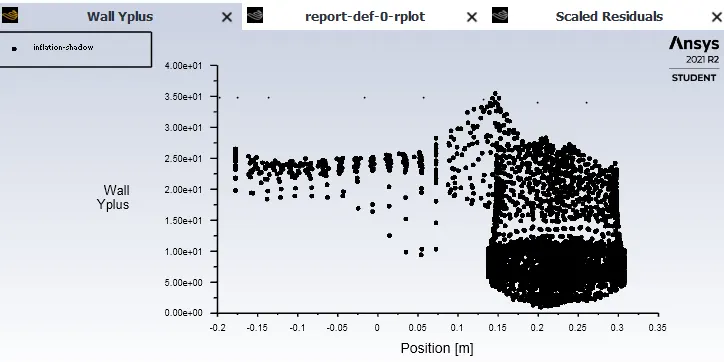
Fig. 17 Y-plus 30 (the maximum value greater than 30)

CASE 2

Turbulence model= k-epsilon

element size=20mm,

max. element size = 100mm

elements =356131

Y-plus =30

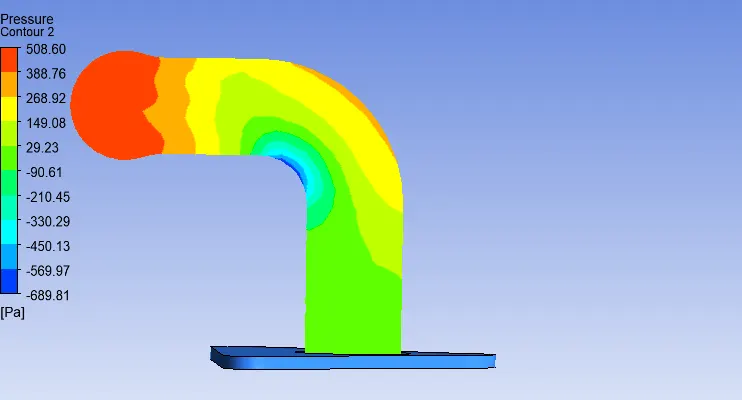
Fig. 18 Pressure contour (element size=20mm)

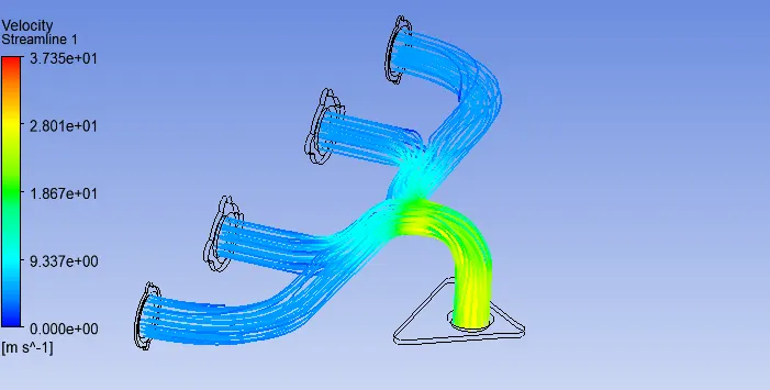
Fig. 19 Velocity streamline (element size=20mm)

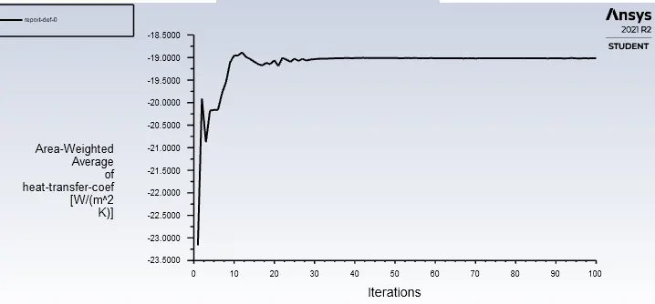
Fig. 20 area weighted average of heat transfer coefficient Vs iteration

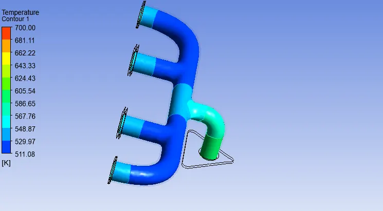
Fig. 21 Temperature contour(element size=20mm)

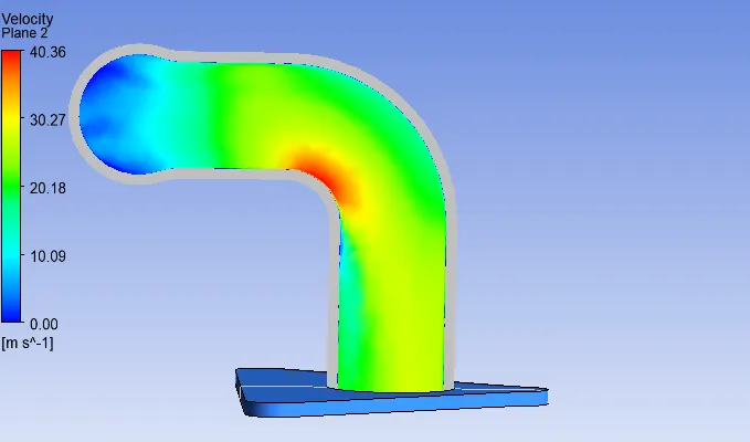
Fig. 22 Velocity plane (element size=20mm)

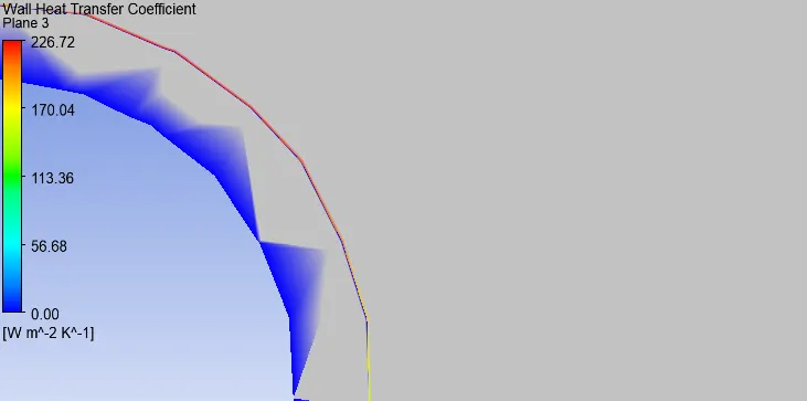
Fig. 23 wall heat transfer coeficient (element size=20mm)

CASE 3

turbulence model=k-epsilon

element size=100,

max. element size = 150mm

Y-plus=100,

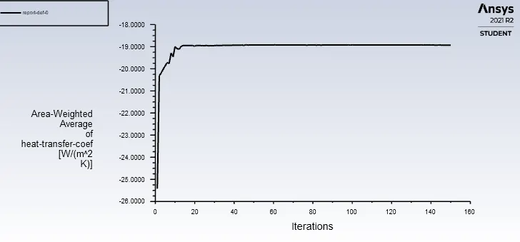
Fig. 24 area weighted average of heat transfer coefficient Vs iteration

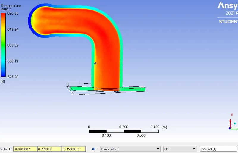
Fig. 25 plane showing temperature variation

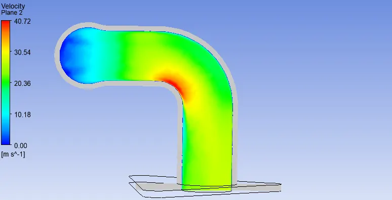
Fig. 26 plane showing velocity distribution

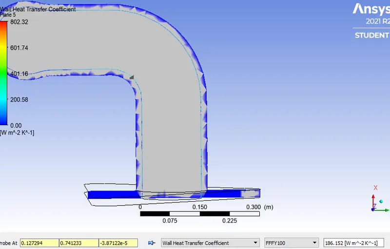
Fig. 27

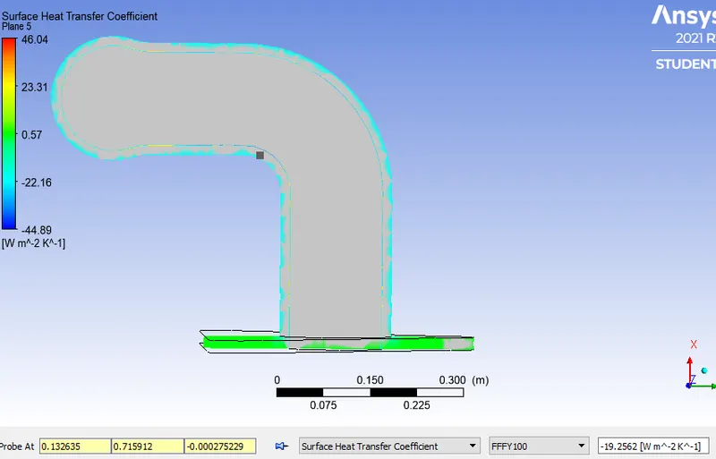
Fig. 28

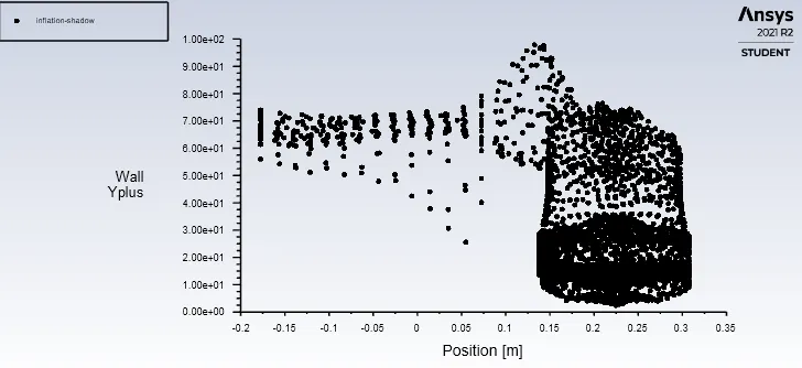
Fig. 29 Y-plus 100

• Here the values are under 100 and the majority values are below 5, So,Y-plus 100 using k-epsilon turbulence model depicts the surface htc and wall htc(local values) near to the correlation values.

CASE 4

Turbulence model =k-omega

element =274403

max. element size = 100mm

element size= 100mm

Yplus =10

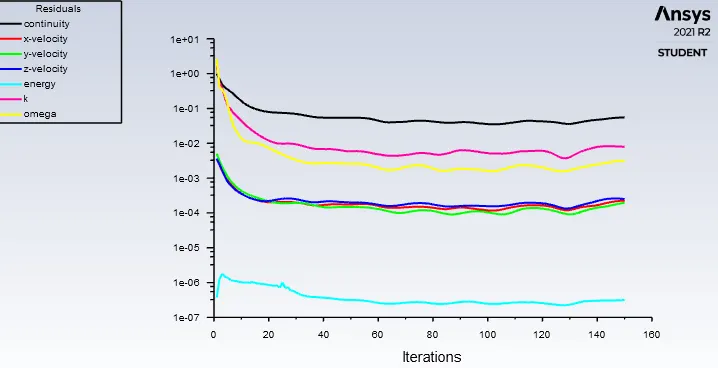
Fig. 30 Residual Vs iteration

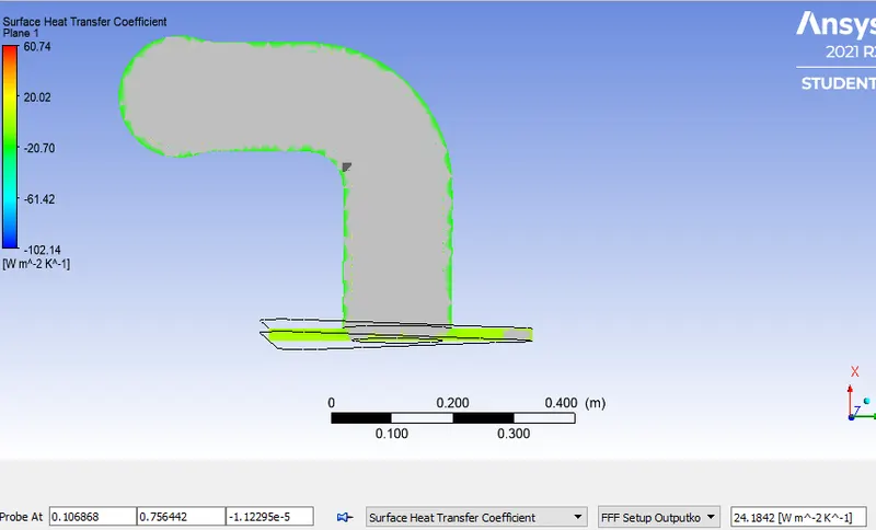
Fig. 31 surface heat transfer coeficient

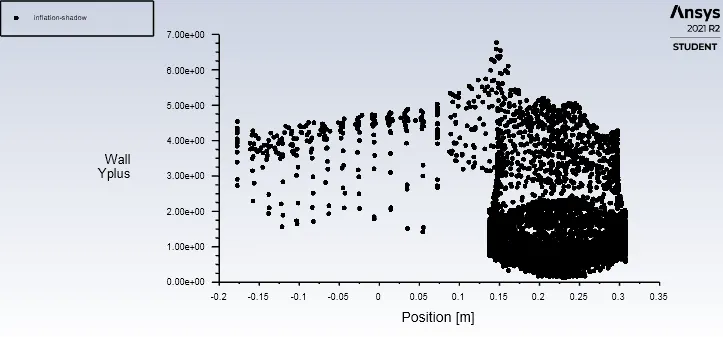
Fig. 32

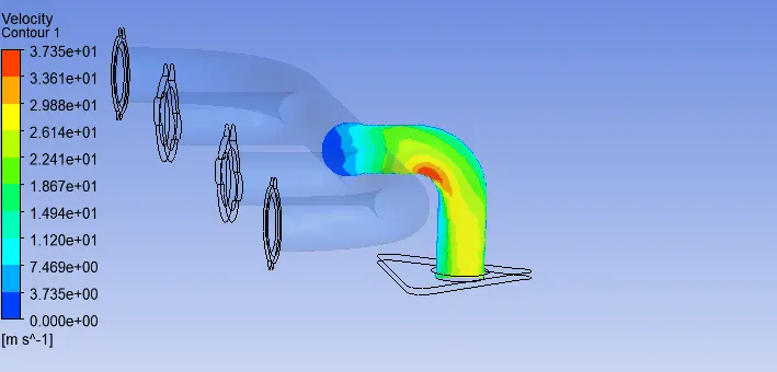
Fig. 33 Velocity Contour

Fig. 34 Velocity streamline

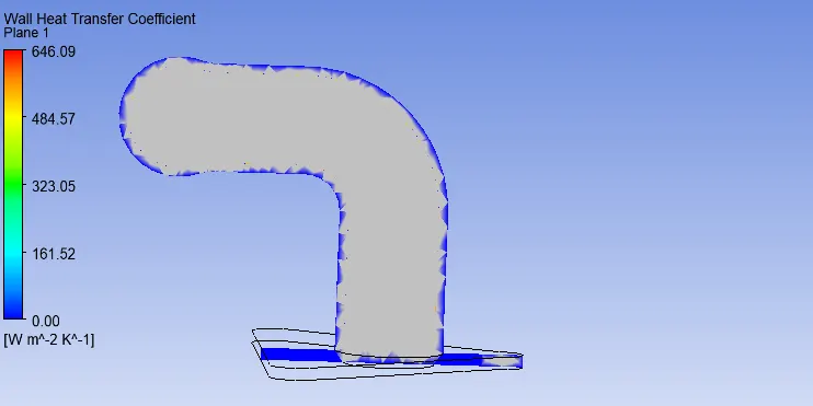
Fig. 35 Wall heat transfer Coefficient

CASE 5

Turbulence model =k-omega

element =456596

max. element size = 30mm

element size= 18mm

Yplus =5

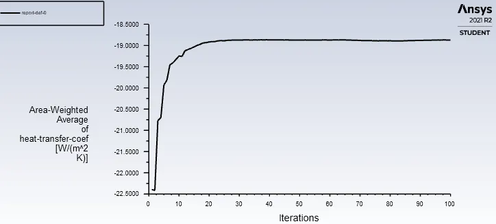
Fig. 36 Area weighted average of heat transfer coefficient Vs iteration

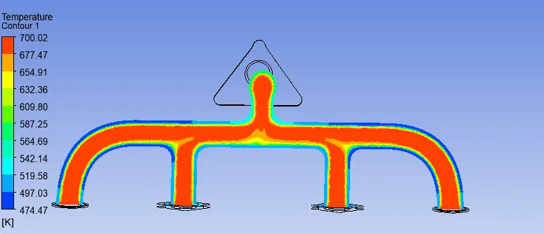
Fig. 37 Plane showing Temperature magnitude

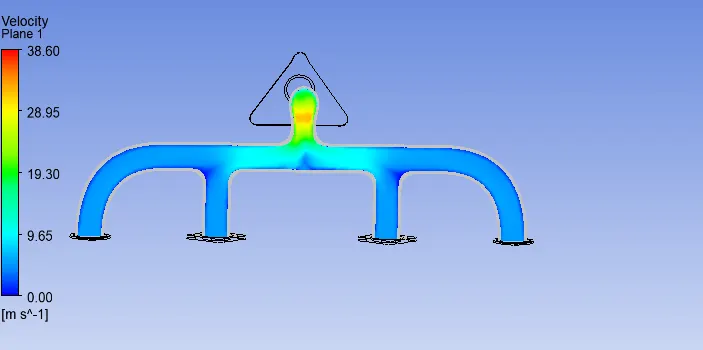
Fig. 38 Plane showing Velocity magnitude

• Here the velocity of exhaust gases coming out of exhaust valve of respective cylinder is found to be having increased flow velocity near to the exhaust manifold as due conservation of mass principle.

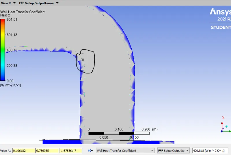
Fig. 39 Wall heat transfer coefficient

• As the Y-plus value increases the center to center distance of cell increases.So, the temperature difference increase and hence the htc decreases.

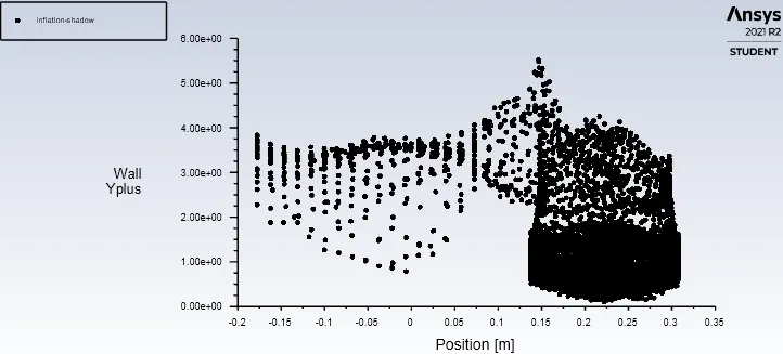
Fig. 40 Y-plus 5

CASE 6

Turbulence model =k-omega

element =456596

max. element size = 30mm

element size= 20mm

Yplus =3

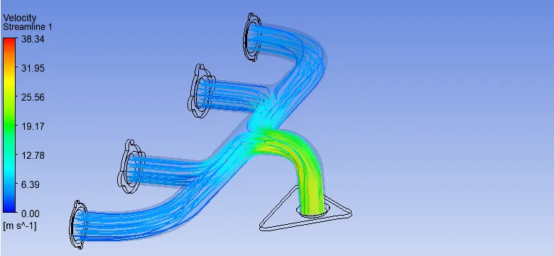
Fig. 41 Velocity streamline

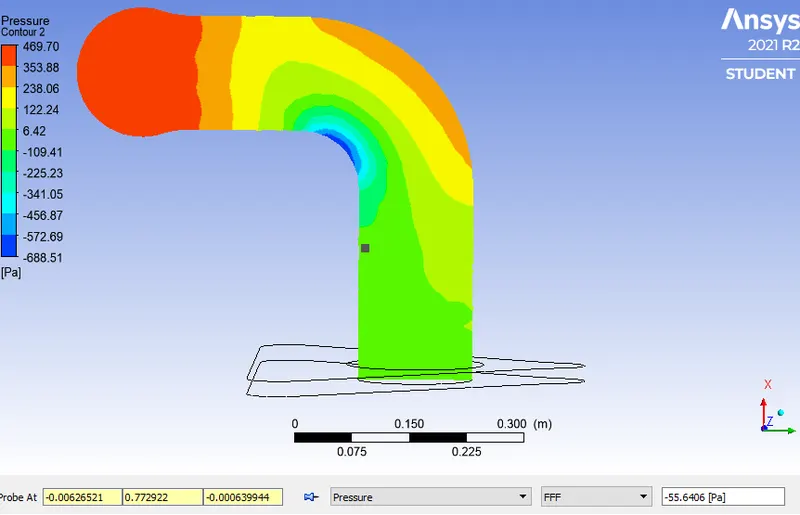
Fig. 42 pressure contour

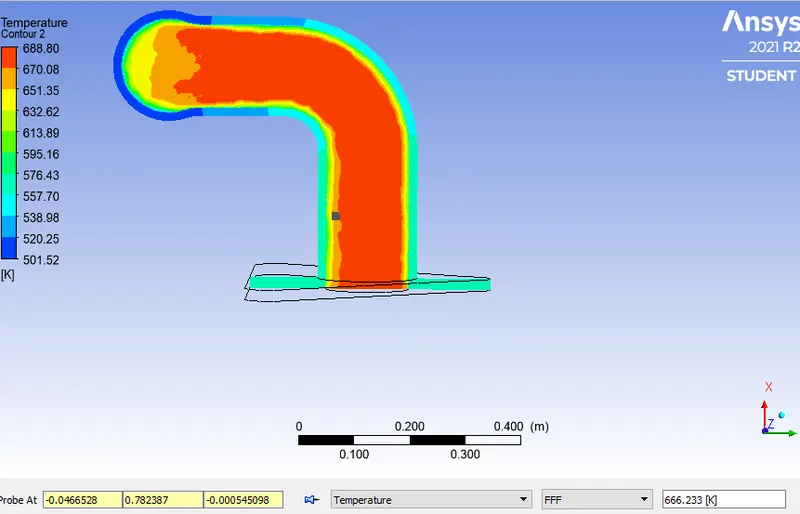
Fig. 43 Temperature Contour

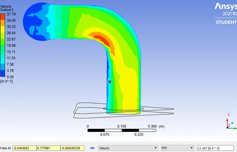
Fig. 44 Velocity Contour

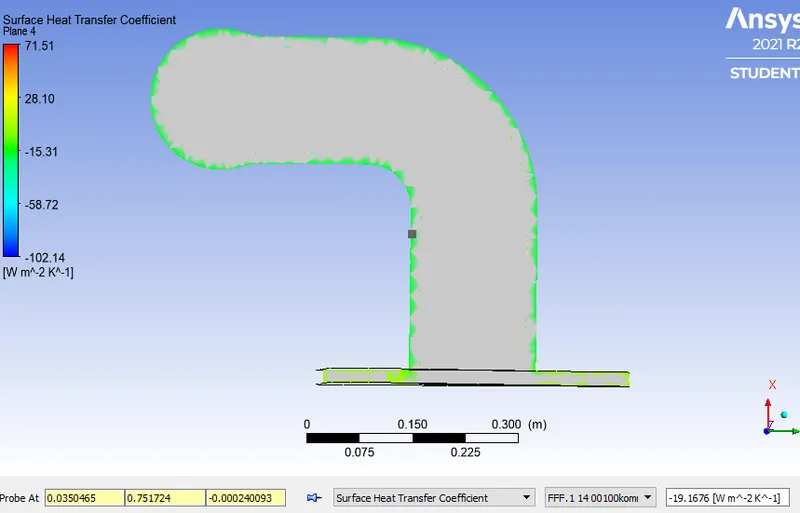
Fig. 45 Surface heat transfer coeficient

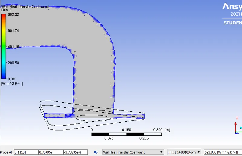
Fig. 46 Wall heat transfer Coefficient

• Here the probe shows the value of internal wall heat transfer coefficient as 693.876(local) where the velocity is maximum.This might be the reason of inflation layer i.e, the total thickness is 0.5mm(very close to the wall).

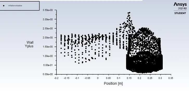
Fig. 47 Y plus 3

Here the plot shows the maximum number of points lies below 3 but maximum value is around 3.25. So, the simulation is correct according to mesh element size.

DITTUS-BOELTER EQUATION

• The correlation for Nusselt number for internal flow (turbulent case) is given by : `N_u=0.023*Re^(0.8)*Pr^(1/3)`

Prandtl number for air is taken as 0.7

• `Nu=126` ( correlation result`)

• For calculating the Reynolds number, we have `Re=(rho*velo*dia)/mu`
  

Re= (5*0.17*1.225)/(1.872*10^(-5))

=`5.56*10^(4)`

As we know for calculating the thickness of 1st layer for inflation layer is given by : `Y=(Y^+ *mu)/(V_f*rho)`

• friction velocity =`sqrt((tau_w)/rho)`=`sqrt(0.07885/1.225)`=`sqrt0.0643`=0.2535

• skin friction coefficient =`(2*tau_w)/(rho*velo^2)`
• wall shear stress= `0.5*C_f*rho*velo^2`

• skin friction coefficient= 0.079*Re^(-0.25)=0.079*0.065299=0.00515
• wall shear stress = 0.5*0.00515*1.225*25 =

• Y= `(Y^+*1.872*10^(-5))/(0.2535*1.225)`

Y-PLUS	Y	total thickness
100	6.02mm	14.97 mm
30	2.21mm	5.49mm
10	0.6mm	1.5mm
5	0.3	0.76
3	0.18	0.447mm

• From the above plots it is observed that , surface heat transfer is calculated more precisely in k-omega model whereas the wall heat transfer coefficient (inside the exhaust pipe) is giving better results in k-epsilon model.

Calculation

• Nu= `(hl)/k_f`= (20*0.17)/0.024 =141.66 (analytical result)

K-air =0.025 at 300k

L(characteristic length, diameter of inlet exhaust)= 0.17m

q=8215.25 (w/m^2)

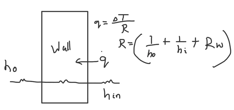
Rconvective = `1/(h_i)+1/(h_o)+L/k`=`1/20+(0.015/202)+1/(h_i)`

heat flux= `q=(DeltaT)/(R_(conv)`=`366.223/(0.05+1/(h_i)+0.000123`

`h_i=1/0.0052981`=188.75` analytical result

• we are getting the wall heat transfer coefficient as approximately as 186.15 from the simulation result ( k-epsilon model,Y-plus 100,element size 100mm) as the local region where the velocity maximum , the htc supposed to be maximum. So, a probe is taken at this location to measure the htc value.

element size	number of elements	Turbulence model	Yplus	inflation total Thickness	surface Heat Transfer Coefficient ( simulation)	Wall heatTransfer Coefficient
100mm	262428	k-epsilon	30	5.49mm	19.99	226
20mm	356131	k-epsilon	30	5.49mm	18.92	226
100mm	274403	k-omega	10	1.5mm	19.015	332
100mm	276227	k-omega	5	0.8mm	18.66	420
18mm	456596	k-omega	3	0.5 mm	18.80	693
100mm	260755	k-epsilon	100	14.9 mm	18.92	186.15

• The accuracy of predicting the heat transfer coefficient depends on:

1. size of mesh element
2. y-plus value for turbulent model
3. inflation layer
4. choosing right turbulent model say k-omega or k-epsilon.

CONCLUSION

• The velocity of hot exhaust fluid increases near the exit. All the fluid streams get mixed near the exhaust port.
• The k-epsilon turbulence model predicts more accurate results for wall heat transfer. For heat transfer coefficient inside the manifold shows the variation as more turbulence is captured. As we move towards the center line of exhaust manifold, the 'h' value is stabilsed. For k-omega model, it is capturing the thermal boundary layer more precisely as the Y-plus value is less than 10. This model shows higher wall heat transfer coefficient.
• K-epsilon model satisfies the whtc and the correlation values are closer to it.