Week 4 - CHT Analysis on Exhaust port

Objective:

To perform the CHT analysis for an exhaust port of a 4-cylinder inline engine and obtain the heat transfer coefficient on the internal solid surface. Obtain the velocity and temperature contours at an appropriate location.

Introduction:

The exhaust manifold connects the engine cylinder to the muffler collecting the exhaust gases from the cylinder and giving a smooth passage to the muffler. Since the exhaust manifold is the first to encounter high-temperature exhaust gases and it works under the harsh condition of the alternating state between high temperature and the normal temperature which might lead to thermal fatigue cracking, fracture, and leakage. The working process of the exhaust manifold is a complex conjugate heat transfer (CHT) problem of fluid-solid coupling.

Conjugate heat transfer problems are encountered in many practical applications, where heat conduction in a solid region is closely coupled with convection heat transfer in an adjacent fluid region. A few examples are the heat transfer enhancement with a finned surface, heat transfer in a cavity with thermally conducting walls, cooling of micro-electronic chips, heat transfer in the workpiece and so in.

Geometry Preparation:

The geometry preparation takes place in the following steps:

1. Import the geometry.

2. Extract the volume of fluid.

This procedure is done to extract the fluid volume portion so that it can be differentiated between the solid volume (pipe) and the fluid volume (air).

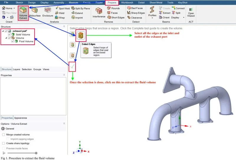
3. Create a new component from the extracted fluid volume and the solid volume.

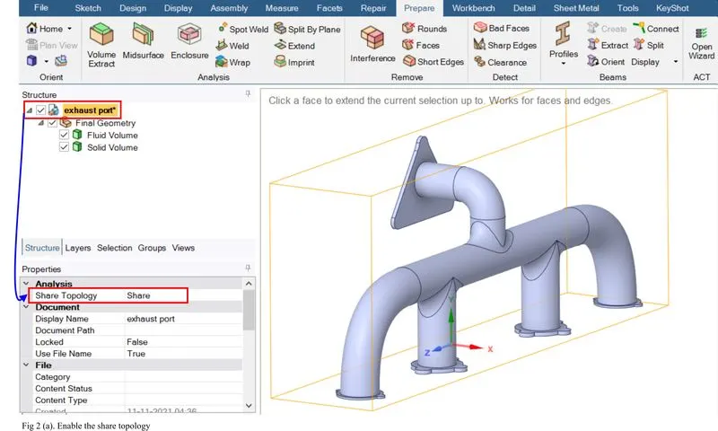
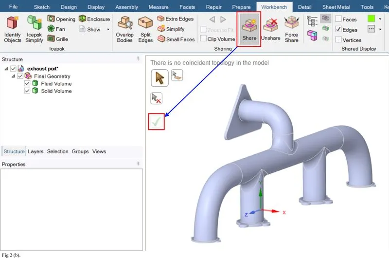
4. Share Topology

This problem requires solving the governing equation across the interfaces. So this procedure is performed to ensure that all the information can be shared across the interface without any discontinuity.

Grid Generation:

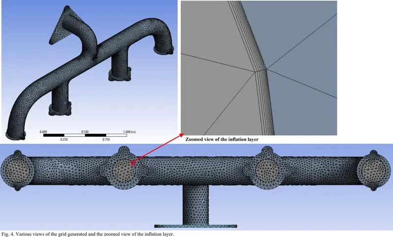
The geometry in the present study is a little bit complex in nature so it is not possible to generate body-fitted grid points in the entire domain. Also, the flow is turbulent in nature so the grid should be fine enough to capture the variation of flow field variables. So to encounter this problem inflation layer is used. Using the inflation layer one can generate a body-fitted grid near the wall up to a certain number of layers of grid points.

But the question is how to decide the first layer thickness of the inflation layers?

The value of the first layer thickness is determined using the value of y+. The value of y+ depends upon the turbulence model that is being used to model the problem.

The range of y+ is as follows:

0<y+<5 is for the k-omega turbulence model;

30<y+<300 is for k-epsilon turbulence model.

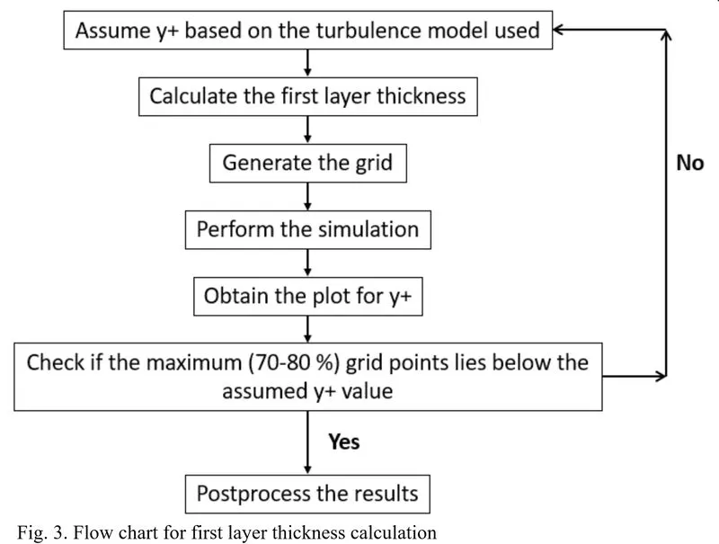
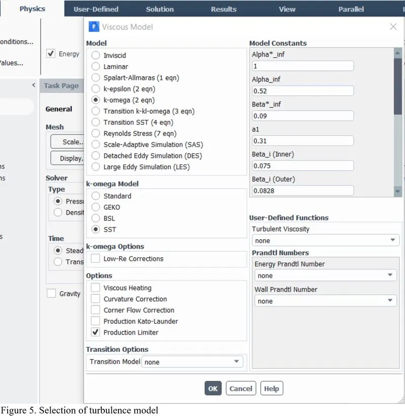
For the present study, the `k-omega` turbulence model is being used, and the value of y+ = 1.

The grid generated is shown in fig. 4 with the zoomed view of the inflation layers.

Problem physics set-up:

1. As the flow is turbulent, so to solve this `k-omega` turbulence model is being used along with the energy equation.

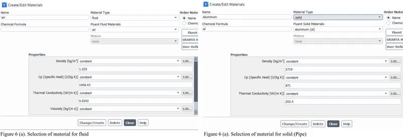
2. Selection of material for the fluid and the solid which is the pipe itself.

3. Setting up the boundary condition:

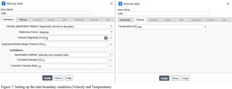
At the inlet, the velocity is set to 5 m/s and the inlet temperature of the hot fluid from the exhaust is 700 K, as shown in fig. 7.

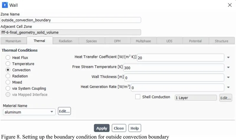
At the outlet, the default pressure-based boundary condition is defined which is 0 gauge pressure at the outlet. While another boundary which is the outermost layer of the pipe, the convection-based boundary condition is defined. The outermost layer of the pipe interacts with the ambient and transfers the heat with the help of convection. In this study, a heat transfer coefficient of `20(W)/(m^2.K)` is assigned.

4. Selection of solution method.

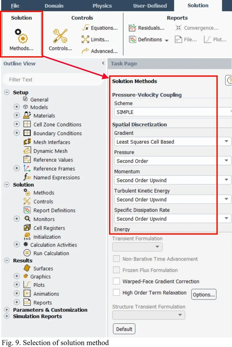
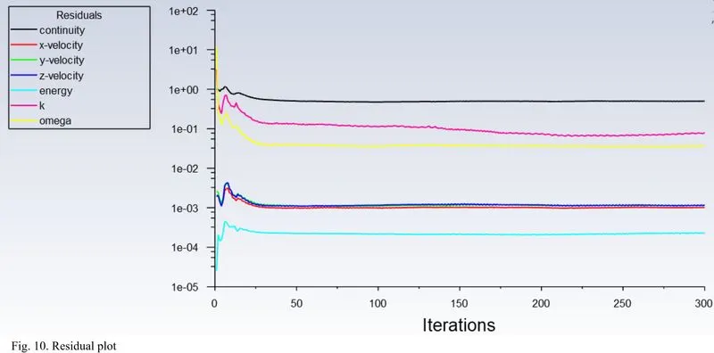
So, once the solution method is selected, initialization of variables is performed and then the calculation is performed. For the present case, the calculation is performed for 300 iterations. However, it is being observed from the residual plot that the steady-state is being achieved after approximately 70 iterations.

Now the plot for y+ is obtained to validate the assumed y+ value which was considered at the time of grid generation to determine the first layer thickness.

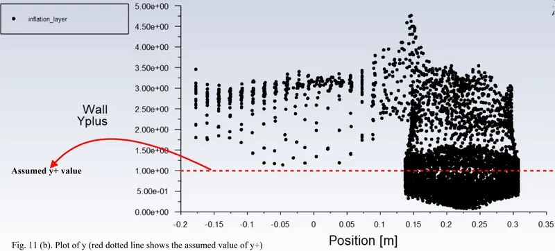
So it is clear from the fig 11 (b), that most of the grid points lie below the assumed y+ value and the maximum value of y+ is less than 5 which is the upper limit of y+ for the `k-omega` turbulence model.

Results:

Once the simulation is performed the following plots is being obtained:

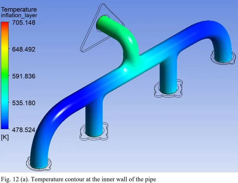
Fig. 12 (a) shows the variation of the temperature in the inner wall of the pipe. At first instance, this temperature plot seems to be counter-intuitive because at the wall the temperature is minimum at the inlet of the exhaust port while it is maximum at the outlet of the port. So, to explain this variation, the plot of the heat transfer coefficient is being obtained on the inner wall of the pipe as shown in fig. 12 (b).

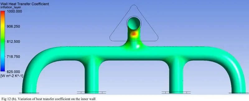
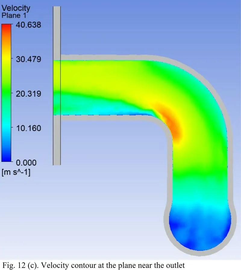
So, it is clear from the plot of heat transfer coefficient that it is minimum near the inlet of the port while it is maximum near the outlet of the port and that is the temperature is higher near the outlet of the port rather than near the inlet of the port. The heat transfer coefficient depends upon the thermo-physical properties of the fluid, the flow passage (length scale), and the velocity of the fluid through the passage. In this case, there is 4 inlet of the exhaust gas while there is a single outlet whose diameter is approximately equal to that of the inlet, so the velocity will be higher near the outlet (from conservation of mass) which is the reason for the high heat transfer coefficient. Fig. 12 (c), shows the variation of velocity near the outlet of the port.

Conclusion:

1. The temperature of the inner wall of the pipe attain maximum near the outlet of the exhaust port while it has a minimum value near the inlet of the exhaust port.

2. Heat transfer coefficient on the inner side of the pipe is higher near the outlet of the exhaust port while it is minimum near the inlet of the port.

References:

1. A note on the solution of the conjugate heat transfer problems using SIMPLE-like algorithms, Xi Chen, Peng Han, International Journal of Heat and Fluid Flow, 463-467, March 2000.

2. https://www.pointwise.com/yplus/index.html. (For the calculation of first layer thickness of the inflation layer based on y+).