CHT Analysis on Exhaust port
OBJECTIVE:-
- To understand the concept and its importance of Conjugate Heat Transfer (CHT) and also its applications.
- Simulate Exhaust port model in ANSYS FLUENT Software while maintaining the Y+ value in the Turbulence Model and also calculate the Heat transfer coefficient on the internal surface.
- Do the Heat transfer coefficient Validation that simulations are correct.
Contents:-
- Concept of Conjugate Heat Transfer (CHT)
- Modelling and Solving approach.
- Validation of HTC
1: Concept of CHT:-
Where and Why CHT analysis is used?
The Conjugate Heat Transfer (CHT) analysis type allows for the simulation of heat transfer between solid and fluid domains by exchanging thermal energy at the interfaces between them. In solids, conduction often dominates whereas in fluids, convection usually dominates. Conjugate heat transfer is observed in many situations. For example, heat sinks are optimized to combine heat transfer by conduction in the heat sink with the convection in the surrounding fluid.
Heat Transfer in Solids - In most cases, heat Transfer in fluids due to conduction that is described by Foureris law defining the conductive heat flux, q, proportional to the temperature gradients: 
Heat Transfer in Fluids - In most cases, heat Transfer in fluids due to convection that is described by Newton's law of cooling defining heat flux, q, proportional to the temperature difference: 
Where and Why CHT is used conjugate Heat Transfer analysis:- HVAC, Heat exchanger ,Boiler, Heat pipe, Tank, Internal combustion engine, Heat sink and Turbocharger.
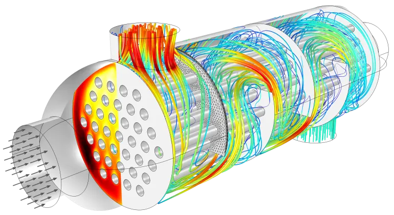
Shell and Tube type heat exchanger
Efficiently combining heat transfer in fluids and solids is the key to designing effective coolers, heaters, or heat exchangers.The fluid usually plays the role of energy carrier on large distances. Forced convection is the most common way to achieve high heat transfer rate. In some applications, the performances are further improved by combining convection with phase change (for example liquid water to vapour phase change).Even so, solids are also needed, in particular to separate fluids in a heat exchanger so that fluids exchange energy without being mixed.
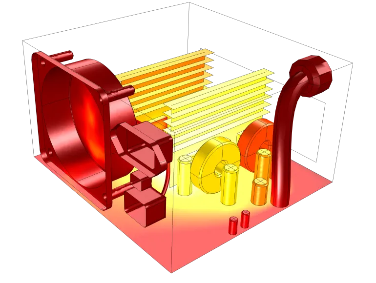
here, is another example of CHT Heat sinks are usually made of metal with high thermal conductivity (e.g. copper or aluminum). They dissipate heat by increasing the exchange area between the solid part and the surrounding fluid.
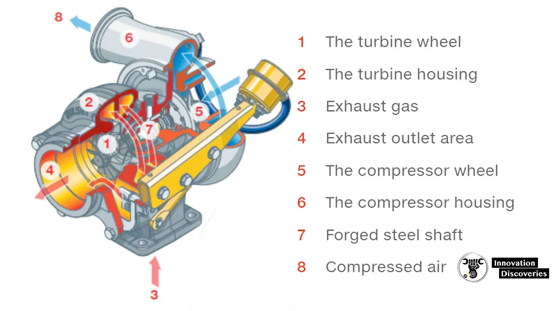
Turbocharger
The air entering a diesel engine is compressed before the fuel is injected. This is where the turbocharger is critical to the power output and efficiency of the diesel engine. It is the job of the turbocharger to compress more air flowing into the engine’s cylinder. When air is compressed the oxygen molecules are packed closer together. This increase in air means that more fuel can be added for the same size naturally aspirated engine. This then generates increased mechanical power and overall efficiency improvement of the combustion process.
Advantages of CHT:-
- Temperature Distribution analysis.
- Temperature distribution analysis.
- Heat flux rate analysis – calculation of wall heat flux rates or heat transfer coefficients.
- Visualisation of heat transfer features for improved understanding of system flow phenomena.
- Identification of localised ‘hot spots’ or heat sinks in checking against specified requirements.
- Evaluating variation in temperature peaks for different operating conditions/ failure modes.
- Assessing insulation or heat shield effectiveness and optimising of material selections.
- Coupling CHT with FE analysis to evaluate thermally induced stresses, expansion or fatigue.
- Temperature field analysis
- CFD thermal analysis
- Heat transfer coefficient analysis
- Heat transfer rate analysis.
2: Modelling Approach:
There is a solid model of Exhaust port in which 4 Cylinders are inligned. There are both conduction and convective heat is transfered by both forced and natural convection method. We are simulating CHT analysis in exhaust port in which we are assuming hot fluid is passed through the 4 cylinders and solid pipe is heated by this fluid from inside and we are going to calculate the heat transfer coefficient of internal Solid surface.
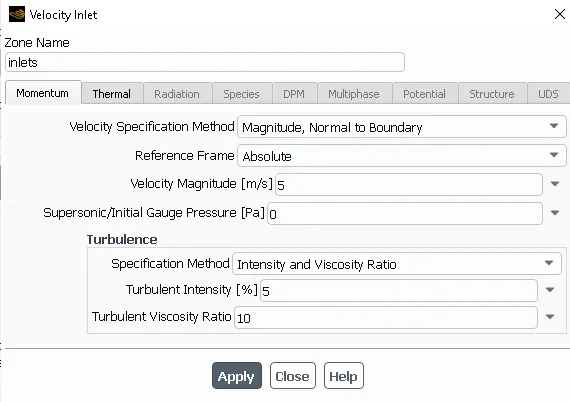
The inlet velocity velocity is giving 5 m/s with thermal conditions temperature = 700 k and the Outlet at open air pressure. The open air has heat transfer coefficient = 20 w/m^2k and the thin flim temperature is 324.34 k.
Solving Approach:-
Create or Import Geometry in Spaceclaim and Meshing
Outlet diameter = 150mm
Inlet of each diameter = 166mm
Wall thickness = 15mm
no. of inlets = 4
Outlet = 1
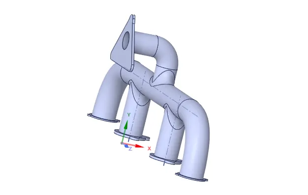
- Import Geometry and extract Voume.
- Share Topology to avoid non-confirmal mesh.

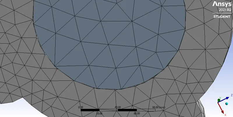
- Confirmal mesh is important for CHT analysis because we want this to overlap perfectly means heat is transfered from fluid to soid.
- Rename as solid-vol and fluid-vol and edit to new component and delete the empty components.

- Go to Workbench and select shareprep to share the interference.
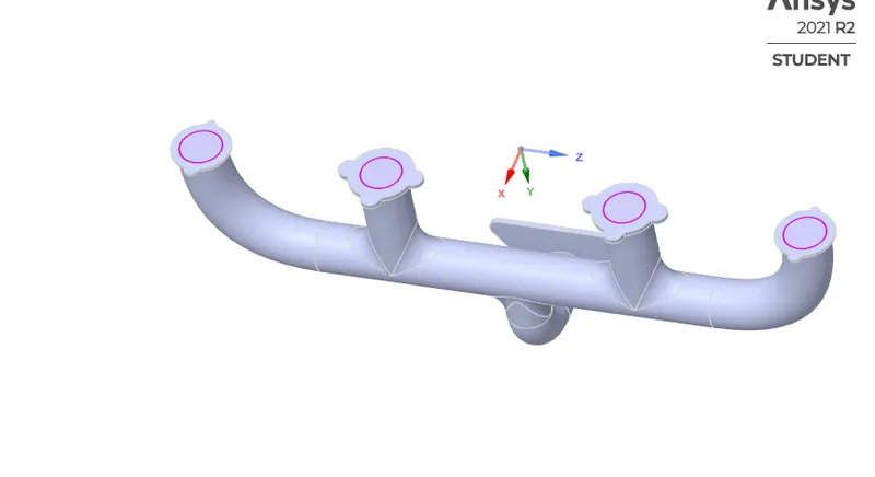
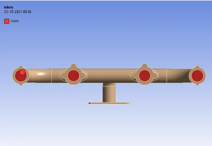
- Close spaceclaim and start mesh then named selection command is used to give the boundaries names as
Inlets
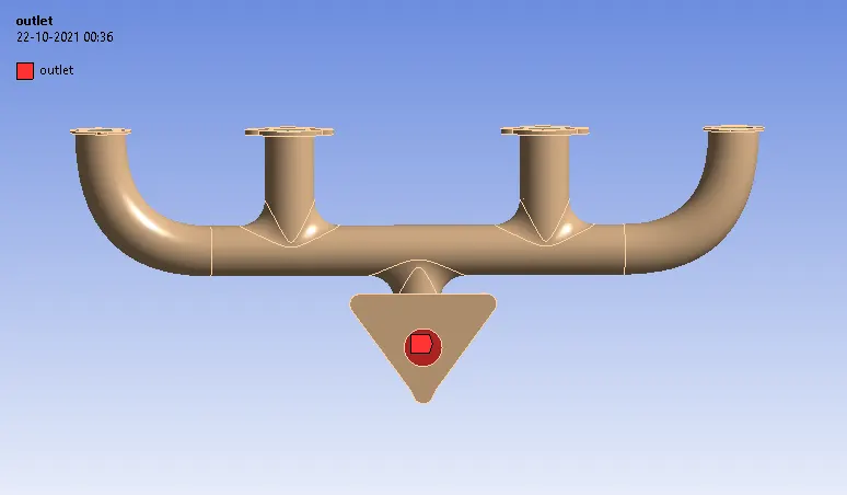
Outlet
Outer-wall
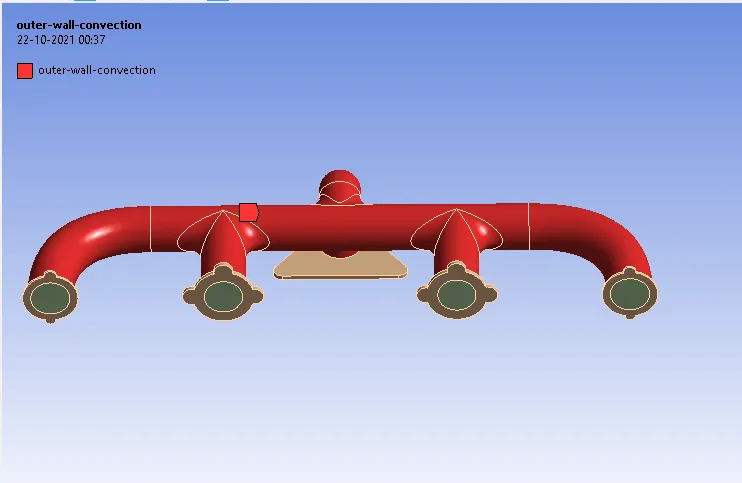
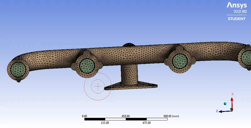
This problem is solved by using two methods one is having a Baseline mesh with element size = 150mm and no. of element are 136424 and the second one is Refined mesh. We are here going to explain the Refines mesh procedure as baseline mesh is simple we just give the element size as we want and then generate the Mesh.
- For Refined mesh In this case we are given the element size = 25mm and no. of elements are 251115.
- Go to Insert>sizing and then select the solid body and then give the element size = 25mm
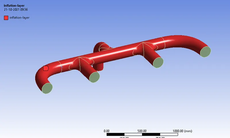
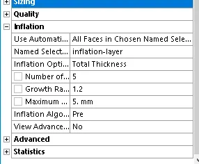
- For adding Inflation layer first we have to add the boundary name called inflation-layer by selection the fluid-vol part and then use type- total thickness and give the total thickness as 5mm. Curvature capture is yes and Then generate Mesh.
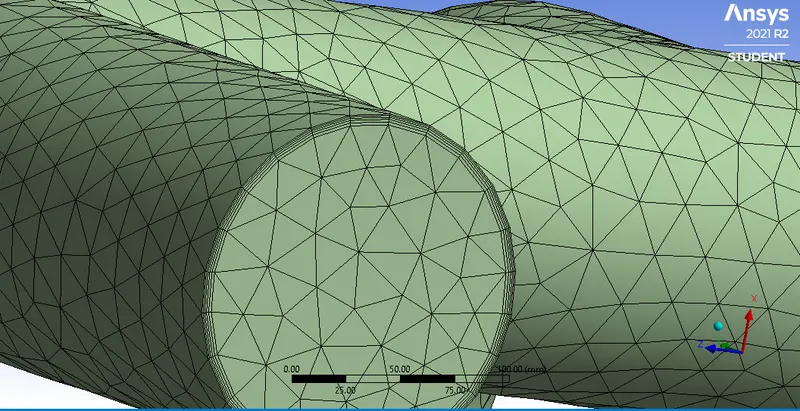
Final mesh
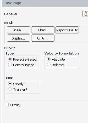
Start a FLEUNT Setup
- Match the Zone names and then click on apply. Reload the data.

- Solver we are using in this case - Pressure-Based steady state.
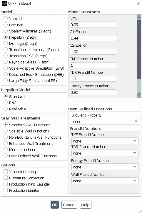
- Turbulence Model - K Epsilon.
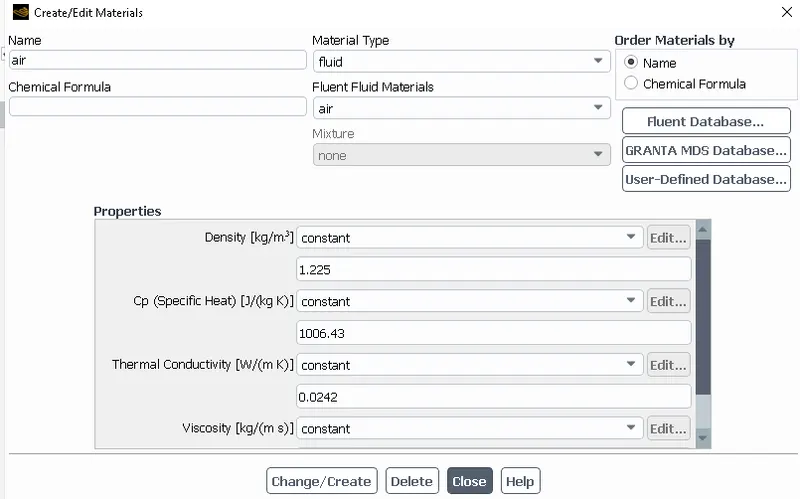
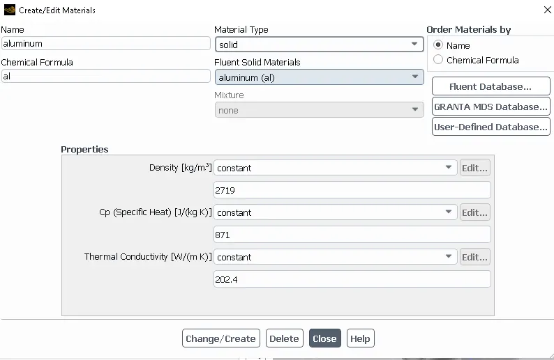
- Material selection: Material selected for solid is Almunium and for Fluid is Air
- Boundary conditions settings at diifferent sections are given as follows:
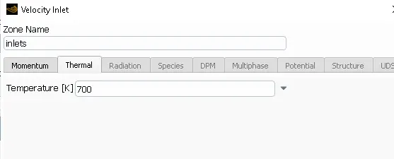
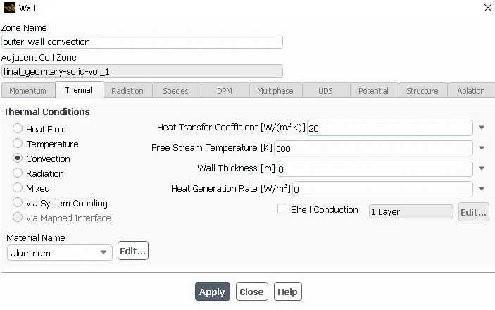
- Initilazation - Hybrid because It provides very good initial conditions.

- Then we are going to set up for Contour Plot of Temperture and Report of Heat Transfer coefficient.
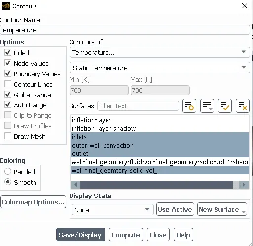
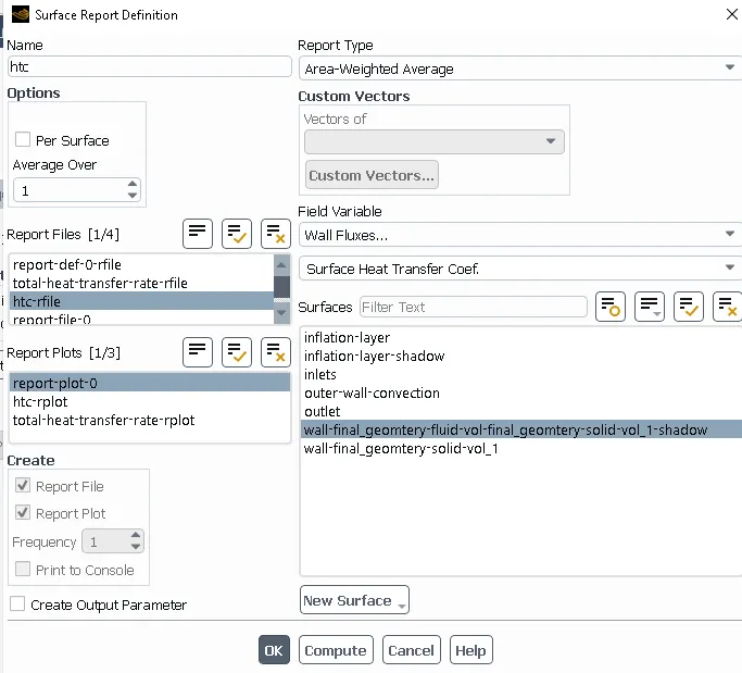
- Then Hit calculate and here are the Results
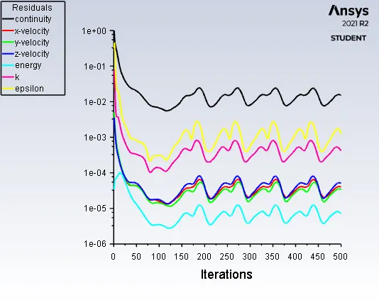
case 1 : Results For baseline mesh of element size = 150mm with no. of elements are 136424, turblence model is K-epsilon model.
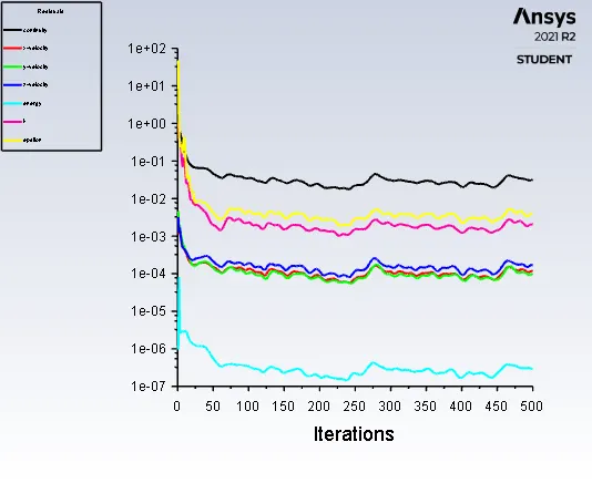
Residual Plot
Area-weighted -Average plot
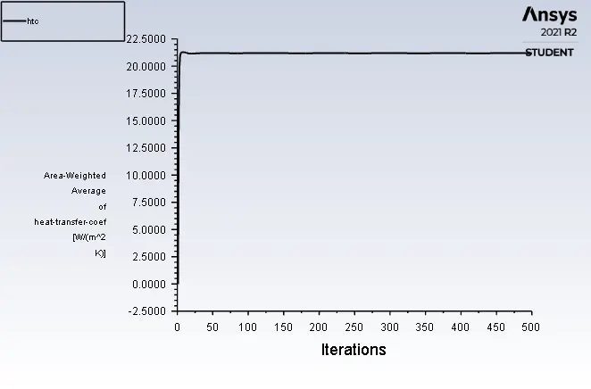
Here we are calculating the average of Heat Transfer Coefficient beacuse it is vary over the entire field as the heat flux and temperature varies over a surface So, if you want single value of heat transfer coefficient we have to area-weighted-average. In this case we got average on the internal surface HTC = 21.178 W/m^2K
PostProcessing (Results)
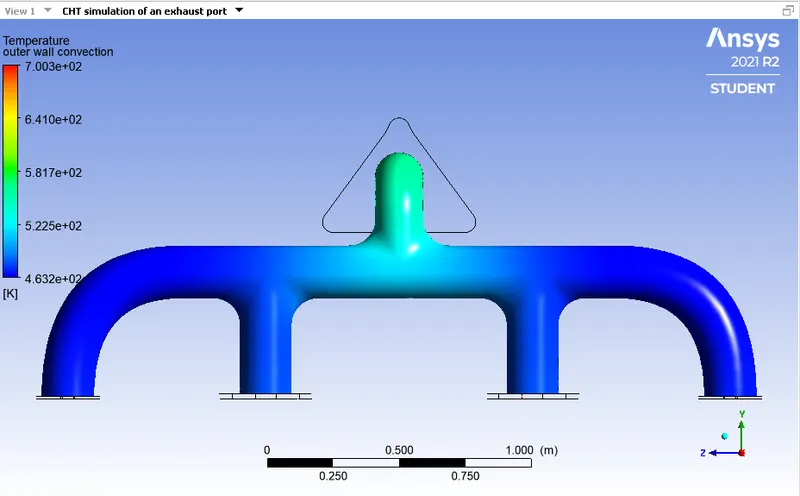
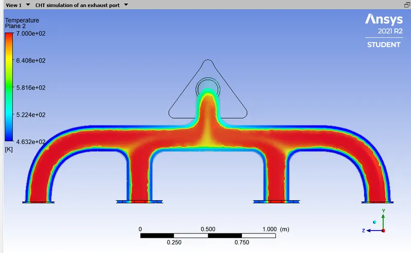
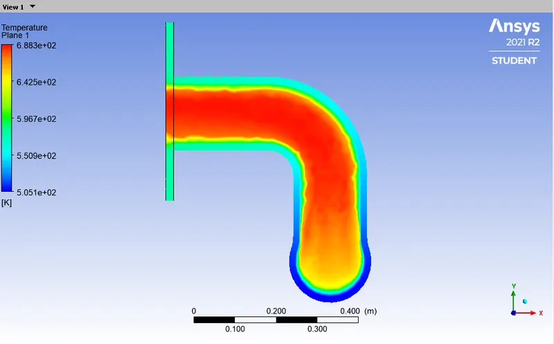
Temperature Contour in YZ plane
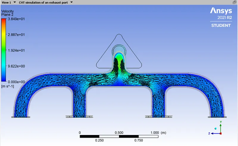
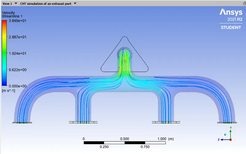
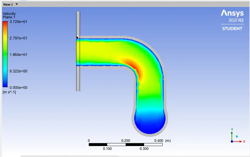
Velocity contour in YZ plane
Temperature and Velocity Contours in XY plane
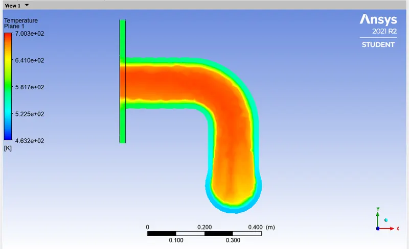
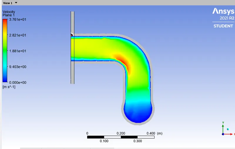
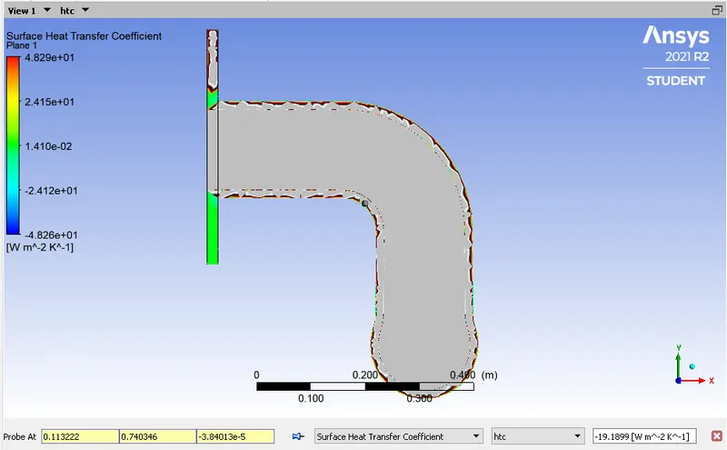
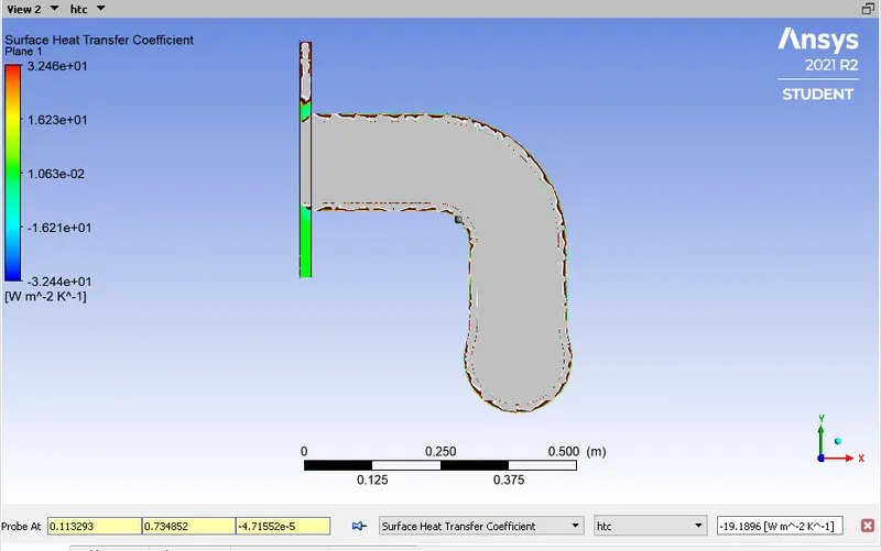
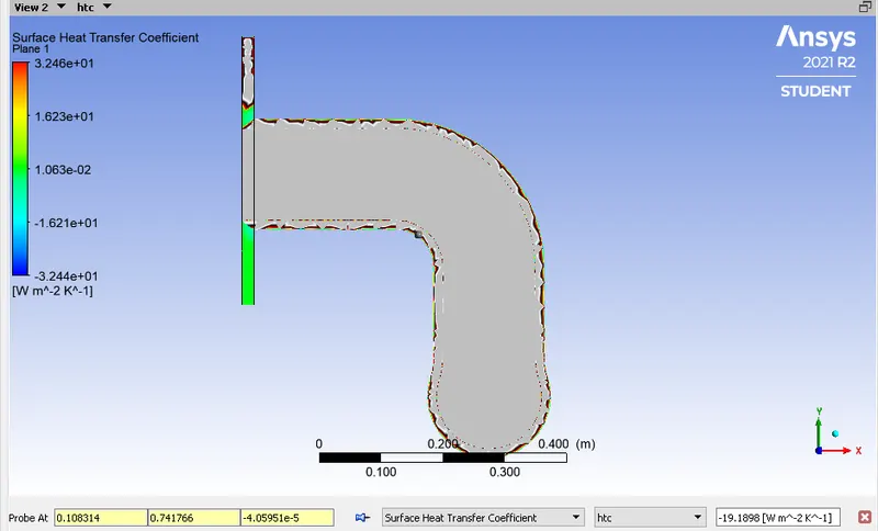
Surface Heat Transfer Coefficient
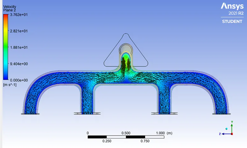
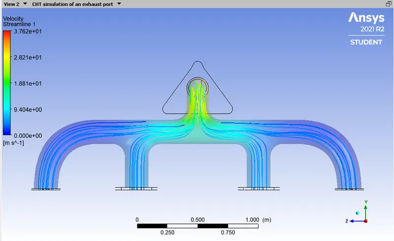
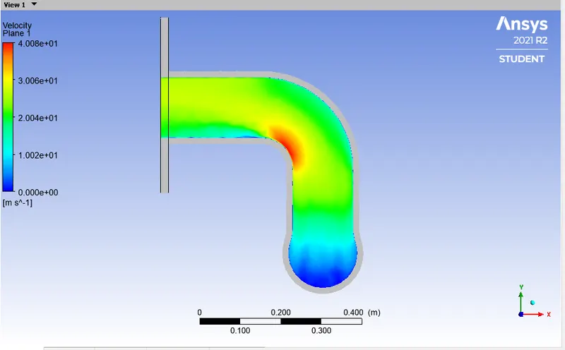
Here, we can clearly see that the velocity at the outlet is very high as compared to the velocity at the inlets is very low It is because of mass conservation law. According to conservation law The rate flow at the inlets = The rate flow at the Outlet
Let us assume A1 = Area at the inlet of cylinder 1, V1 = Velocity at the inlet of cylinder 1
Similarly, A2 = Area at the inlet of cylinder 2, V2 = Velocity at the inlet of cylinder 2
A3 = Area at the inlet of cylinder 3, V2 = Velocity at the inlet of cylinder 3
A4 = Area at the inlet of cylinder 4, V2 = Velocity at the inlet of cylinder 4
A5 = Area at the Outlet, V2 = Velocity at the Outlet
According to the mass conservation law, the Rate flow at the inlets and the Outlet is
A1V1 + A2V2 + A3V3 + A4V4 = A5V5
All the air comes from the inlets needs to coming out from the Outlet means the velocity there is very very high.
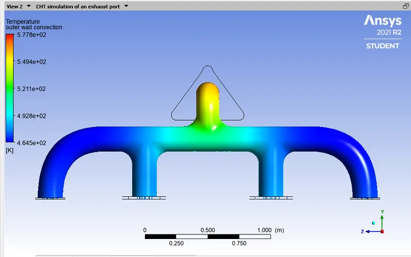
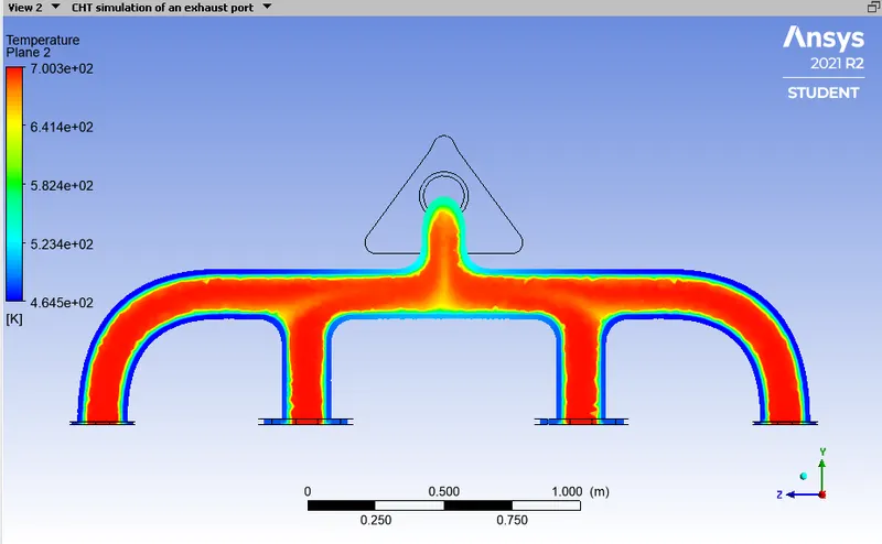
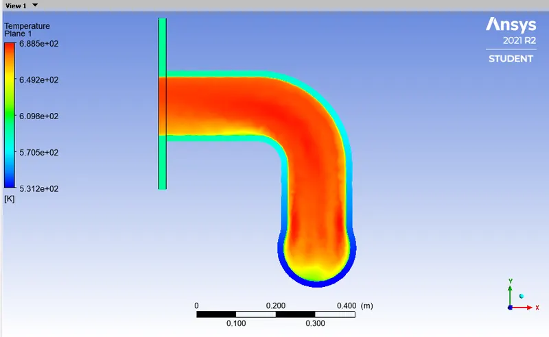
Since, It is Steady state simulation means the air in the Outlet have higher velocity because of higher velocity the Reynold's number is also very higher which means the Heat Transfer Coefficient is also high and the heat should be transfer is more from the fluids to the solids that's why in the Outlet section Temperature is higher.
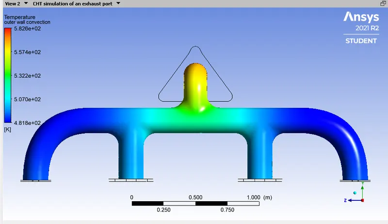
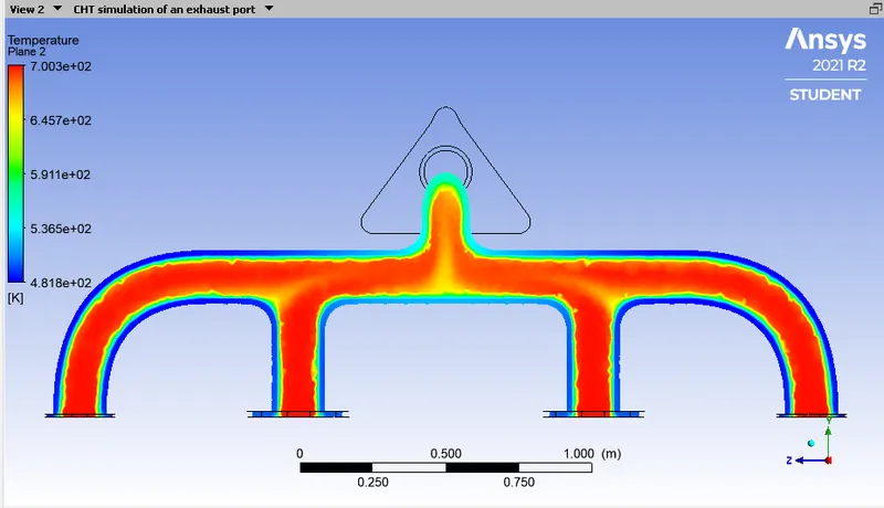
Case 2 : Results For baseline mesh of element size = 150mm with no. of elements are 136424, turblence model is K-omega model.
Residual Plot
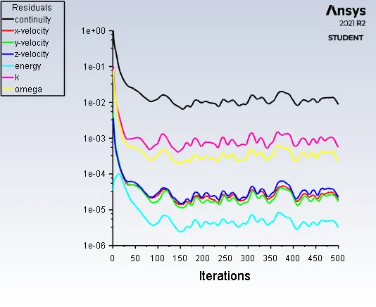
Area-weighted -Average plot
Temperature Contour in YZ plane
Velocity contour in YZ plane
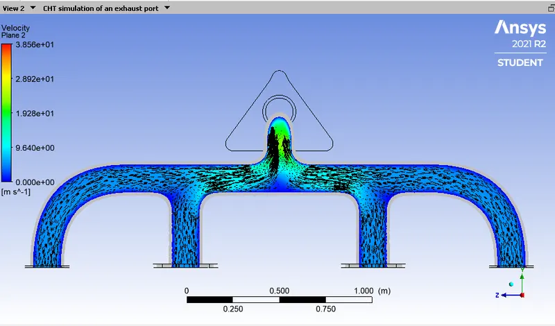
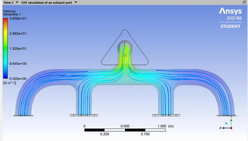
Temperature and Velocity Contours in XY plane
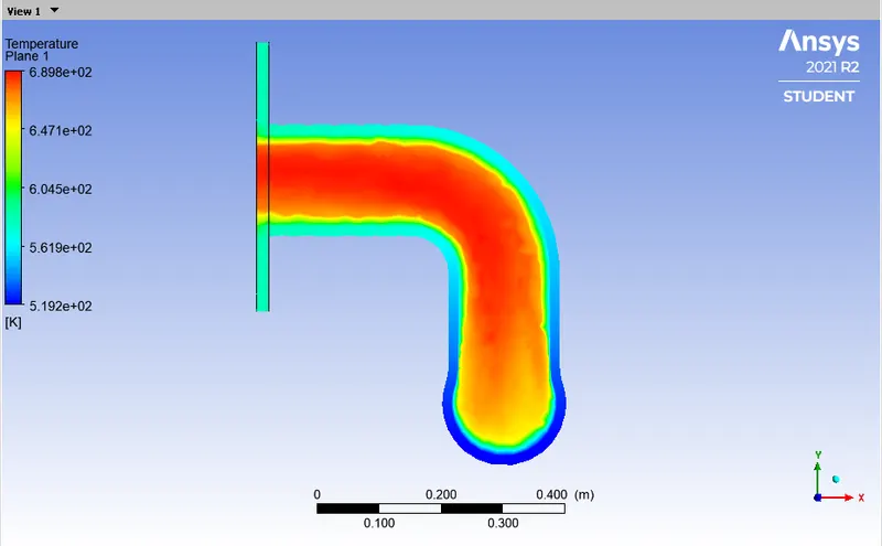
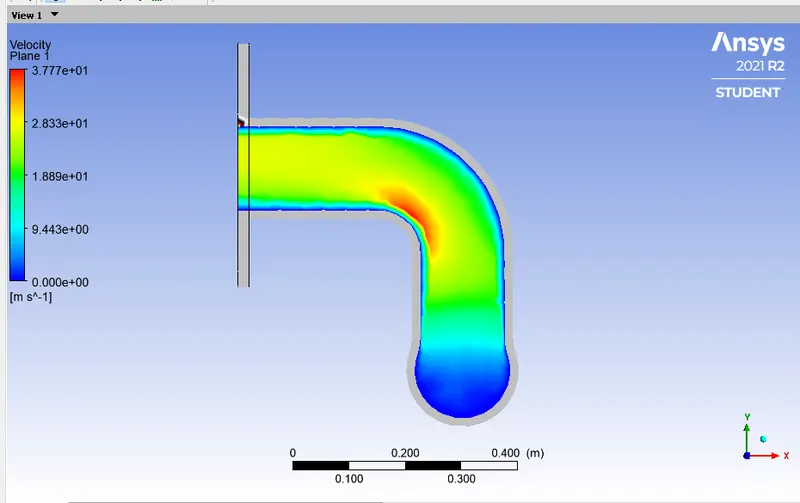
Surface Heat Transfer Coefficient
Case 3 : Results For baseline mesh of element size = 25 mm with no. of elements are 136424, turblence model is K-epsilon model
Residual Plot
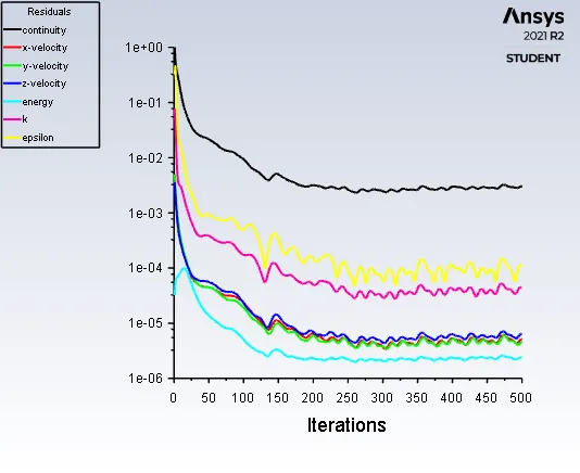
Area-weighted -Average plot
Temperature Contour in YZ plane
Velocity contour in YZ plane
Temperature and Velocity Contours in XY plane
Surface Heat Transfer Coefficient
Case 4 : Results For baseline mesh of element size = 25 mm with no. of elements are 136424, turblence model is K-epsilon model
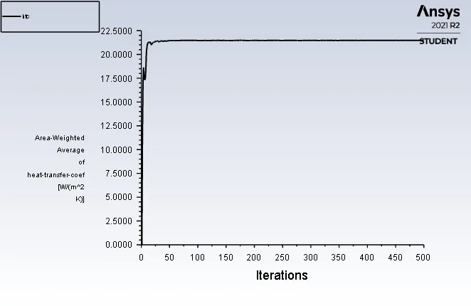
Residual Plot
Area-weighted -Average plot
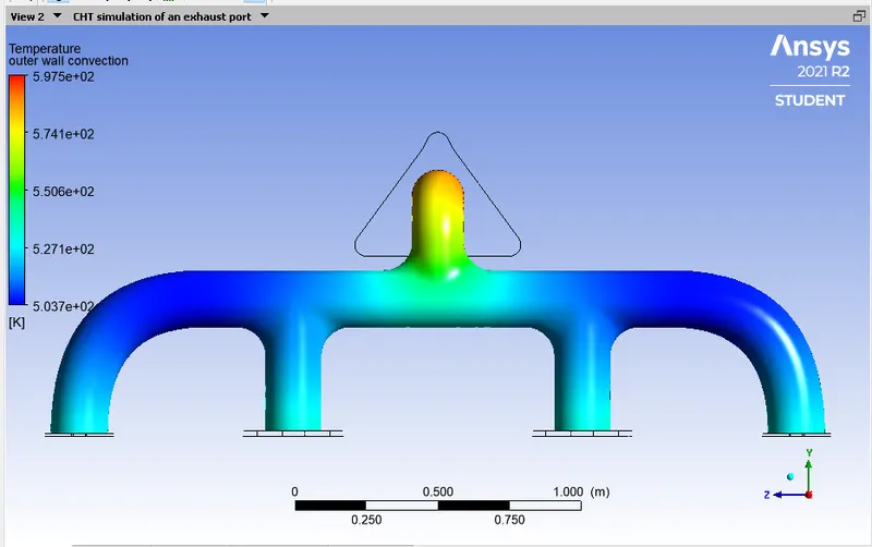
Temperature Contour in YZ plane
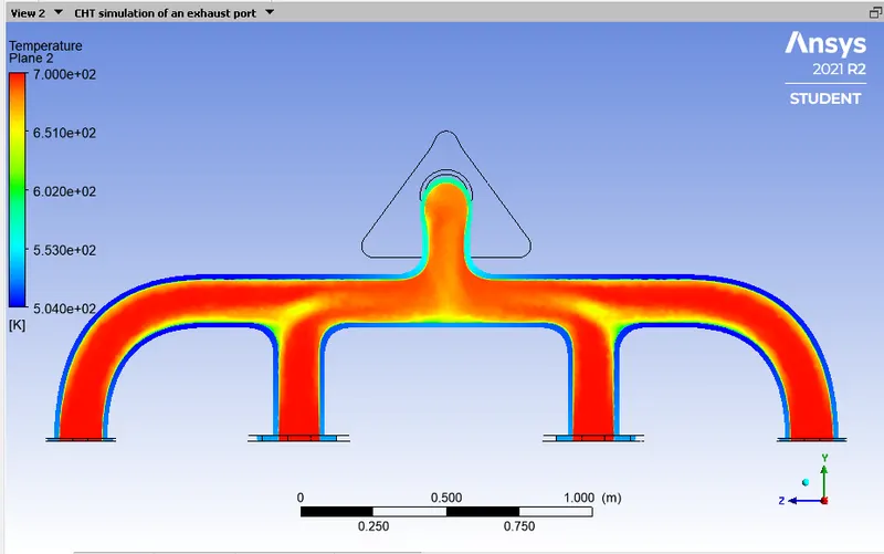
Velocity contour in YZ plane
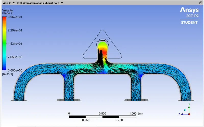
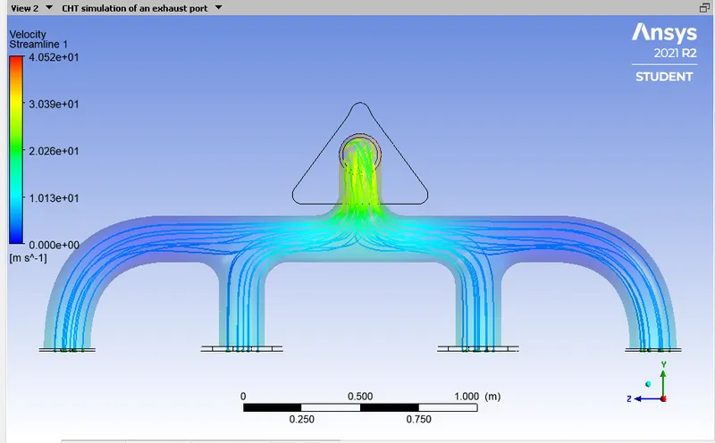
Temperature and Velocity Contours in XY plane
Surface Heat Transfer Coefficient
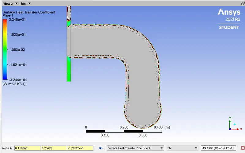
As you see we got the heat transfer coefficient value is negative This happens due to the ANSYS Fluent tells the direction of flow that heat is flowing from Solids to fluids means it is leaving the system. If heat is added to the system the heat flux is represented as positive and vice versa.
Thers are two volumes, Solid and fluid. The heat is flowing from solid to Fluid voume, hence the heat is removed from the system that's why it shows negative value.
From the Output or Plots we are comparing the results,
| Parameter | Max outlet temperature (K) | Max Outlet velocity (m/s) | Surface Heat transfer coeffcient (W/M^2K) |
Average Surface Heat transfer coeffcient value (W/M^2K) |
| Case 1 | 650 | 16.50 | 90.74 | 21.97 |
| Case 2 | 654.96 | 17.44 | 90.31 | 25.39 |
| Case 3 | 660.60 | 15.59 | 86.29 | 21.94 |
| Case 4 | 635.68 | 13.55 | 120.49 | 31.11 |
3: Validation of Heat transfer Coefficient
For Validation of heat transfer coefficient we are going to calculate theortically heat transfer coeffcient to verify since, the heat transfer coefficient is a quantitative characteristic of convective heat transfer between a fluid medium and the surface medium flowed by the fluid. The overall heat transfer coefficient for a multi-layered wall, pipe or heat exchanger - with the fluid flow can be calculating using Nusslet number.
The Nusselt number is the ratio of convective to conductive heat transfer across a boundary. The convection and conduction heat flows are parallel to each other and to the surface normal of the boundary surface, and are all perpendicular to the mean fluid flow in the simple case.
- Nu = (conductive resistance)/(convective resistance)
- `Nu = (L/KA)/(1/hA)`
- `Nu = (hL)/K`
where h is the convective heat transfer coefficient of the flow, L is the characteristic length, K is the thermal conductivity of the fluid.
Example:-Let the Fluid flow over a flat plate with a velocity 5 m/s and length of plate is 1.6 cm and the inlet temperature is 700 k and the ambient temperature is 273K. We are going to validate the heat transfer coeffcient.
Flim temperature = (700+273)/3 = 324.24K
density of air (rho) = 1.225 kg/m^3
kinematic viscosity `(ν) = μ/ρ`
ν = 4.765e-5
`Re = (VL)/ν`
Re = 0.71430e5
Prandtral number (Pr) = (Kinematic viscosity)/(thermal conductivity)
Pr = 0.6935
`Nu = f(Re,Pr)`
Emperical Relationship for flow over a flat plate
`Nu = 0.664*(Re)^0.5 (Pr)^0.34`
(hL)/K = 182.7316
h = (182.7356*K)/0.166 = 222.65 W/m^2K
So, the value is obtained by simulation is near to correct value and this error is minimised by refining the mesh.
Factors on which accuracy prediction depends on :-
- Number of elements in the Meshing means the more finer the mesh the moreyou get the accurate Results.
- Adding Inflation layer around the boundary its like a body fitted mesh gives us most highly accuracy as comparison to the others mesh.
- Accurate fitting of Mesh around the geometry its important because mesh needs to accurately accomodate the geometry around the curvature.
- Setting share topology is more important It gives us confirmal Mesh for transferring of mesh in different zones.
Conclusion:-
From the above simulation plots we can conclude that the by Refining and adding the Inflation layer It gives us the accurate results. Choosing the right Turbulence model is also an important role to get the right predictions and also good results. Max surface heat transfer coefficient we got from the good quality, Refined mesh, adding inflation layer and also choosed correct turbulence model is about 120 W/m^2k. So these factors are most important to get the actual results.