Week-4 Challenge WOT Condition Part-2

1. What is the difference between mapped and dynamic model of engine, motor and generator? How can you change model type?

Solution :

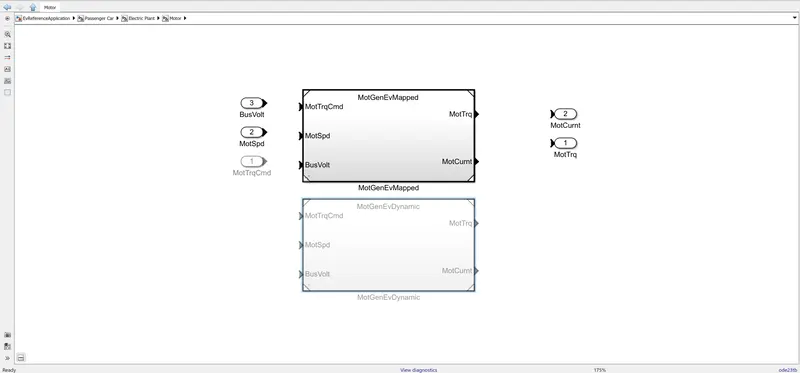
Mapped Model :

The Mapped Motor block implements a mapped motor and drive electronics operating in torque-control mode. The output torque tracks the torque reference demand and includes a motor-response and drive-response time constant.

We can specify:

• Port configuration — Input torque or speed.
• Electrical torque range — Torque speed envelope or maximum motor power and torque.
• Electrical loss — Single operating point, measured efficiency, or measured loss. we can virtually calibrate the measured loss tables.

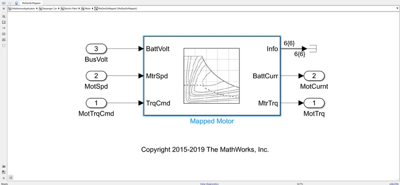
• BattVolt - Battery voltage, in V.
• TrqCmd - Commanded motor torque, in N·m.
• MtrSpd - Motor shaft speed, in rad/s.
• BattCurr - Battery current draw or demand, I_batt, in A.
• MtrTrq - Motor output shaft torque, in N·m.
• Info — Bus signal - following bus calculation (mechanical power, internal inverter and motor power loss, electrical power and motor power loss).

Characteristics :

1. Mapped motor operates with the pre-assigned values given in the look up table.
2. The output motor torque generates a value without considering the real time engine or motor parameters.
3. The out put values are stored in corresponding input parameters.
4. The accuracy of this type of simulation is not as high as it does not consider real time values.

Dynamic Model :

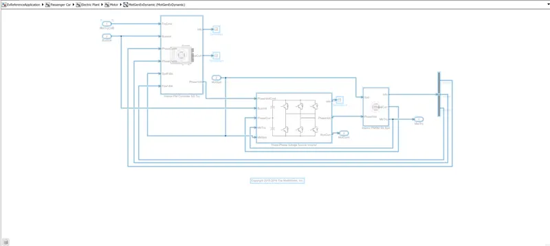
Three Phasse Voltage Source Inverter :

Implements a three-phase voltage source inverter that generates line-to-neutral voltage commands for a balanced three-phase load. Configure the voltage switching function for continuous voltage or inverter switch input signals. To enable electrical loss calculations suitable for memory optimized code generation, select Enable memory optimized 2D LUT.

Interior PMSM :

Model the dynamics of a three-phase interior permanent magnet synchronous motor (PMSM) with sinusoidal back electromotive force.

Interior PM Controller :

Implements a torque-based, field-oriented controller for an internal permanent magnet synchronous machine (PMSM) with an optional outer-loop speed controller. The torque control implements strategies for maximizing the torque per amp (MTPA) and weakening the magnetic flux.

Characteristics :

1. The dynamic model uses combination of the outputs from various subsystems to arrive at the final output.
2. It runs a real time subsystem, takes input from the specific drive cycle and calculates the result from all the subsystem values.
3. The accuracy of the model is very high as it consider real time values for calculation.
4. The simulation takes along time to complete as the individual subsystems takes their own time to complete each simulation.

Steps to Change the Model Type :

From the power train blockset we get to select the various applications such as below.

Objectives :

1. Design tradeoff analysis and component sizing, control parameter optimization, or hardware-in-the-loop (HIL) testing.
2. Engine and controller calibration, validation, and optimization before integration with the vehicle model.

2. How does the model calculate miles per gallon? Which factors are considered to model fuel flow?

Solution :

• Miles per gallon is a fuel economy rating, and is used to show how far your car is able to travel for every gallon (or 4.55 litres) of fuel it uses.
• Incase of electric vehicles it tells us the energy equivilent to engine power to propel the vehicle to travel a distance.
• In this case the amount of fuel required by the engine to travel a distance is compared to the amount of power required by the battery is compared and arrived at avalue.
• The powertrain blockset has a performance calculation subsystem.
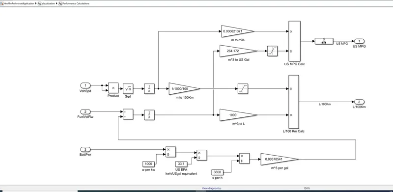
• The below model takes input such as vehicle speed, Fuel flow and Battery power and gives the desired output..

Explanation :

Vehicle speed and Fuel Flow :

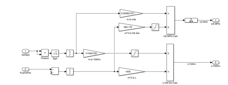
• The vehicle speed is an important parameter which determines the fuel or energy consumption of the vehicle through out the drive cycle.
• In the calculation the distance is found out by integrating the speed to with respect to time, hence integrator is used .
• The fuel flow is the mass flow rate which is calculated as (kg/sec), now integrating flow rate we get total volume of the fuel consumed at particular drive cycle.
• This volume when divided by 1000 we get a value which is in litres.
• And by comparison we get a value which the vehicle runs per 100 km.

Battery Power :

• The amount of energy from battery power required to propel the vehicle equivalent to that of the engine is calculated here.
• The battery power is given in watts and it is converted to KW by dividing by 1000.
• Then we convert the power into energy by multiplying with the time into KWh.
• Then we convert the energy from kwh to equivalent energy in US gallon of automotive gasoline by dividing with 33.7.
• We convert this value to gallon per second by dividing with 3600.
• Then multiplying with 0.00378541 we convert the US Gallons per sec to volume of the fuel flowin (m^3/s) and we multiply with 739(California Phase II gasoline density), which gives the mass flow rate in kd/s.
• Then finally the battery energy equivalent in kg/s is given as a input for the fuel flow parameter in order to find the equivalent Miles per gallon.
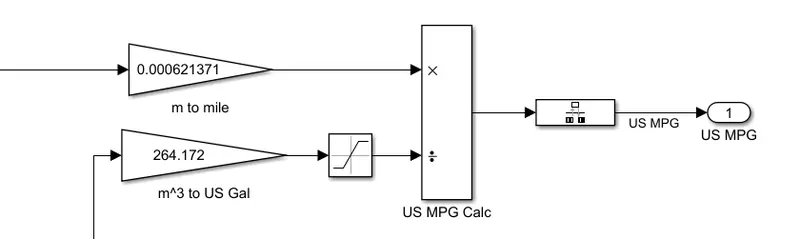
• The inputs from the vehicle speed , the distance we found (in metres) is taken into calculation and it is converted to the miles by multiplying with 0.000621371.
• Then the inputs from the fuel flow (Battery energy +Fuel energy) taken in (m^3) and is converted to equivalent US Gallons by multiplying with 264.172.
• Then the two inputs miles covered and equivalent US Gallon is further divided and the result is got in miles/gallon.

3. Run the HEV Reference Application with WOT drive cycle. Change the grade and wind velocity in the environment block. Comment on the results.

Solution :

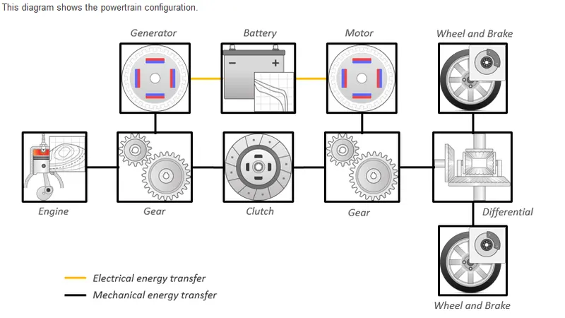
• The hybrid electric vehicle reference application represents a full multimode hybrid electric vehicle (HEV) model with an internal combustion engine, transmission, battery, motor, generator, and associated powertrain control algorithms.
• We use the reference application for powertrain matching analysis and component selection, control and diagnostic algorithm design, and hardware-in-the-loop (HIL) testing.

By default, the HEV multimode reference application is configured with:

• Mapped motor and generator.
• 1.5–L spark-ignition (SI) dynamic engine.

Case 1 :

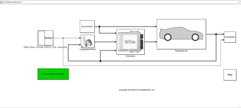
• Drive Cycle Source block - Generates a standard or user-specified drive cycle velocity versus time profile. Block output is the selected or specified vehicle longitudinal speed.
• Environment subsystem - Creates environment variables, including road grade, wind velocity, and atmospheric temperature and pressure.
• Longitudinal Driver subsystem - subsystem -

Uses the Longitudinal Driver or Open Loop variant to generate normalized acceleration and braking commands.

1. Longitudinal Driver variant implements a driver model that uses vehicle target and reference velocities.
2. Open Loop variant allows you to configure the acceleration, deceleration, gear, and clutch commands with constant or signal-based inputs.

• Controllers subsystem - Implements a powertrain control module (PCM) containing a hybrid control module (HCM) and an engine control module (ECM).
• Passenger Car subsystem - Implements a hybrid passenger car that contains engine, electric plant, and drivetrain subsystems.
• Visualisation subsystem - Displays vehicle-level performance, battery state of charge (SOC), fuel economy, and emission results that are useful for powertrain matching and component selection analysis.

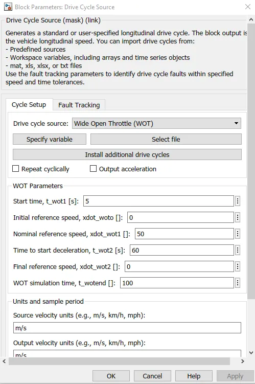
• The drive cycle source taken for this particular simulation is WOT(Wide Open Throttle).
• The nominal reference speed is taken as 50.
• The time to start decceleraton is fixed at 60
• And wide open throttle simulation times is run for 100 seconds.

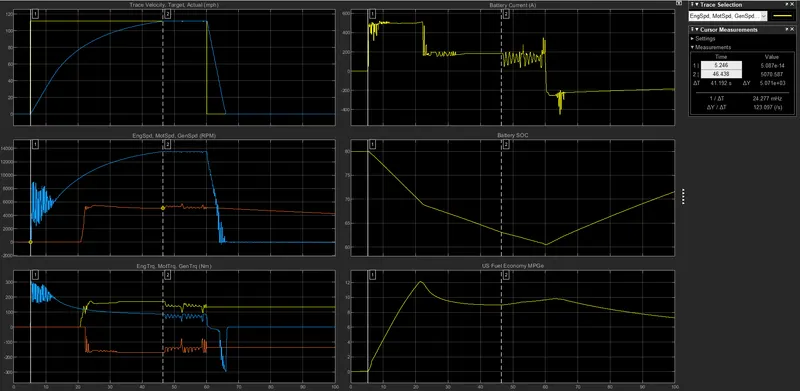
Plot 1 :

• Plot 1 shows the comparison between trace velocity and and actual velocity.
• The time taken for the vehicle to reach maximum acceleration is 41.192 seconds.
• The trace velocity is increasing at a linear rate,then the speed is constant for a period of around 13 seconds.
• The deceleration happens at a time of 60 seconds.
• Then the actual time is constant.

Plot 2 :

• First the motor is starting, hence the motor graph gives us rapid fluctuations.
• Once the motor has started, the generator graph show a significant growth.
• At 54 seconds when vehicle is decelerating the motor power drops and in turn the engine power.
• The generator power remains steady through put the distance.

Plot 3 :

• As motor is starting, hence the motor torque show us a fluctuation at the starting, and gradually becomes steady and at 54 seconds the motor torque drops significantly.
• Once the engine has reached the sufficient Rpm the generator torque decreased, and then becomes steady throghout.
• The engine torque first rises with the starting of vehicle and remains almost constant.

Plot 4 :

• The intake of current by the battery is high, when the vehicle is starting.
• Once it reaches a peak speed the charge input drops.
• At 54 seconds, the while the vehicle is decelerating, the battery current decreases as more more charge is required to recharge the batteries.

Plot 5 :

• SOC means state of charge.
• The state of charge of the vehicle is lowest at 54 seconds.
• The State of charge is the level of charge of an electric battery relative to its capacity.
• As the vehicle ran for its peak value till 41 seconds, the battery ran out.
• Hence the SOC curve has a significant dip.
• Once charged the SOC is recovered again.

Plot 6 :

• The MPG graph shows a steep growth while the vehicle has started .
• The maximum fuel consumption at its peak speed is 12 miles per gallon.
• Once the engine power stabilises the MPG value also decreases and keep on varying with the rpm.

Case -2 :

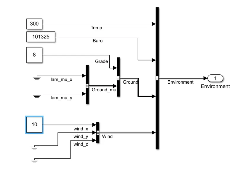
• The gradeability of the sub-system is changed to 8.
• The wind velocity of the system is changed to 10 in the environment block.

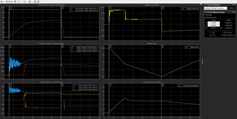
Plot 1 :

• Plot 1 shows the comparison between trace velocity and and actual velocity.
• The time taken for the vehicle to reach maximum acceleration is 54.58 seconds.
• The trace velocity is increasing at a linear rate,then the speed is constant for a period of around 13 seconds.
• The deceleration happens at a time of 60 seconds.
• Then the actual time is constant.

Plot 2 :

• First the motor is starting, hence the motor graph gives us rapid fluctuations.
• Once the motor has started, the generator graph show a significant growth.
• At 54 seconds when vehicle is decelerating the motor power drops and in turn the engine power.
• The generator power remains steady through put the distance.
• The maximum engine rpm is 92.855 rev/min.
• The maximun motor rpm is 152.152 rev /min.
• The maximum generator rpm is 92.855 rev/min.

Plot 3 :

• As motor is starting, hence the motor torque show us a fluctuation at the starting, and gradually becomes steady and at 54 seconds the motor torque drops significantly.
• Once the engine has reached the sufficient Rpm the generator torque decreased, and then becomes steady throghout.
• The engine torque first rises with the starting of vehicle and remains almost constant.
• The maximum engine torque is 3.11 rad/sec.
• The maximun motor torque is 672.105(/ks).
• The maximum generator torque is 3.106 rad/sec.

Plot 4 :

• The intake of current by the battery is high, when the vehicle is starting.
• Once it reaches a peak speed the charge input drops.
• At 54 seconds, the while the vehicle is decelerating, the battery current decreases as more more charge is required to recharge the batteries.

Plot 5 :

• SOC means state of charge.
• The state of charge of the vehicle is lowest at 54 seconds.
• The State of charge is the level of charge of an electric battery relative to its capacity.
• As the vehicle ran for its peak value till 41 seconds, the battery ran out.
• Hence the SOC curve has a significant dip.
• Once charged the SOC is recovered again.

Plot 6 :

• The MPG graph shows a steep growth while the vehicle has started .
• The maximum fuel consumption at its peak speed is 12 miles per gallon.
• Once the engine power stabilises the MPG value also decreases and keep on varying with the rpm.

4. Keeping all other parameters same, compare the simulated results of hybrid and pure electric powertrains.

Solution :

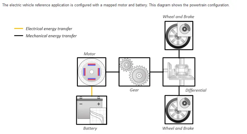
The electric vehicle reference application represents a full electric vehicle model with a motor-generator, battery, direct-drive transmission, and associated powertrain control algorithms.

We use the electric vehicle reference application for powertrain matching analysis and component selection, control and diagnostic algorithm design, and hardware-in-the-loop (HIL) testing.

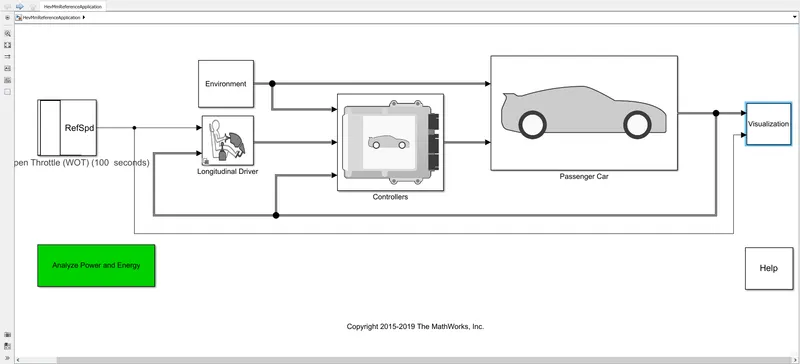
Drive Cycle Source block -Generates a standard or user-specified drive cycle velocity versus time profile. Block output is the selected or specified vehicle longitudinal speed.

Environment subsystem - Generates a standard or user-specified drive cycle velocity versus time profile. Block output is the selected or specified vehicle longitudinal speed.

Longitudinal Driver subsystem -

Uses the Longitudinal Driver or Open Loop variant to generate normalized acceleration and braking commands.

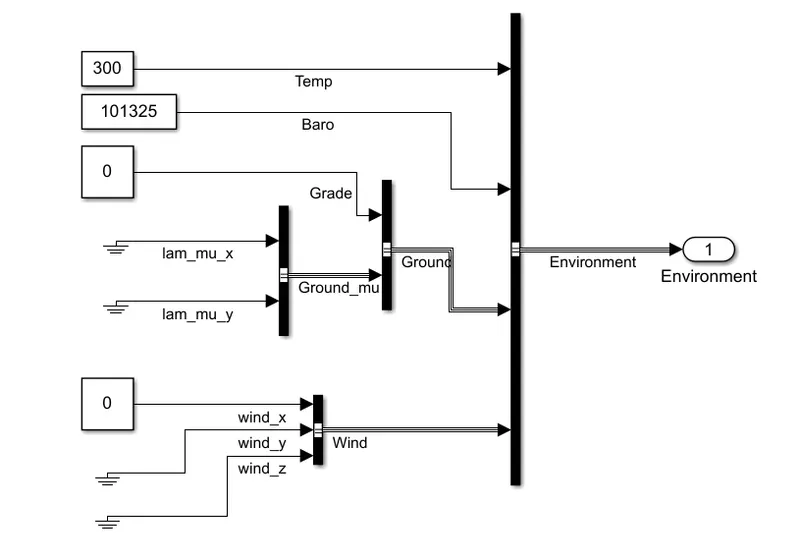
• The grade velocity and wind velocity for the subsystem is kept at 0.

COMPARISON BETWEEN HYBRID AND PURE ELECTRIC VEHICLE.

Electric Vehicle :

Plot 1 :

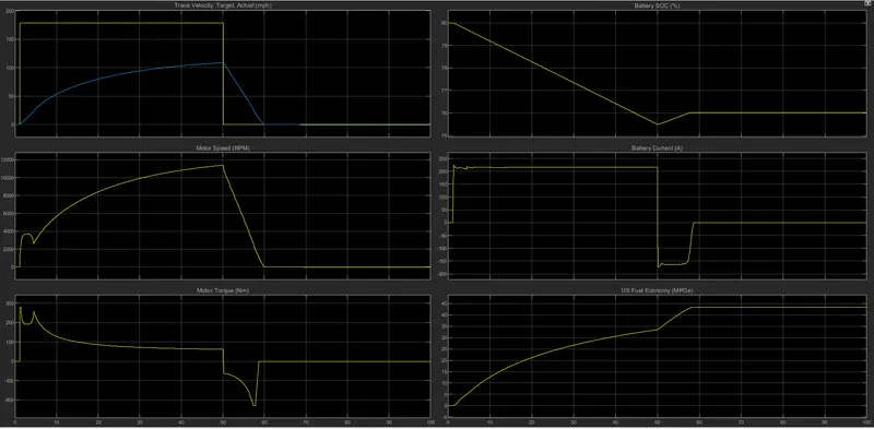
• The plot 1 indicates us the trace velocity and actual velocity.
• The maximum acceleration is attained at 49 seconds.
• The trace velocity has linear values as the drive cycle input is given.
• The deceleration continues till 58 seconds.
• Then the graph becomes steady.

Plot 2 :

• The motor speed increases gradually till 49 seconds because of the engine starting.
• The Rpm falls drastically till 58 seconds as the vehicle is decelerating.
• Then the graph becomes steady for the rest of the simulation.
• The maximum rpm values are 212rad/sec.

Plot 3 :

• The motor torque first increases with the start of the engine.
• Then it decreases gradually as the torque required to run the vehicle is low for the electric vehicle.
• hence at 58 secons as the vehicle decelerates it decreasess more drastically.
• The engine torque is 5.818 Nm.

Plot 4 :

• SOC - State of Charge.
• The state of charge is the level of charge of an electric battery relative to its capacity.
• The soc gets decreased linearly with the vehicle journey as the battery has limited power capacity.
• Then again charging happens and the graph shows a growth and gets constant.

Plot 5 :

• This curve shows us the battery current.
• When the vehicle makes a significant amount of journey the charge gets used up with time, hence the curve drops suddenly when time is 58 seconds.
• And again the battery is charged and the power is replenished.
• Then get constant with reduce of speed.
• The battery current is 3.1 amperes.

Plot 6 :

• This plot shows the miles per gallon consumption of fuel.
• As the vehicle is moving forward the fuel consumption (incase of electric vehicle battery power) is more and increases with a variation.
• Increase with decrease in torque as to keep up with the engine revolution per minute.

Hybrid :

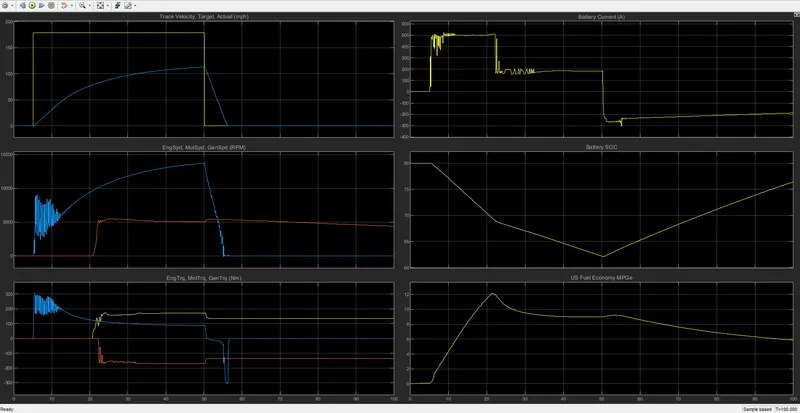
Plot 1 :

• Plot 1 shows the comparison between trace velocity and and actual velocity.
• The time taken for the vehicle to reach maximum acceleration is 41.192 seconds.
• The trace velocity is increasing at a linear rate,then the speed is constant for a period of around 13 seconds.
• The deceleration happens at a time of 60 seconds.
• Then the actual time is constant.

Plot 2 :

• First the motor is starting, hence the motor graph gives us rapid fluctuations.
• Once the motor has started, the generator graph show a significant growth.
• At 54 seconds when vehicle is decelerating the motor power drops and in turn the engine power.
• The generator power remains steady through put the distance.

Plot 3 :

• As motor is starting, hence the motor torque show us a fluctuation at the starting, and gradually becomes steady and at 54 seconds the motor torque drops significantly.
• Once the engine has reached the sufficient Rpm the generator torque decreased, and then becomes steady throghout.
• The engine torque first rises with the starting of vehicle and remains almost constant.

Plot 4 :

• The intake of current by the battery is high, when the vehicle is starting.
• Once it reaches a peak speed the charge input drops.
• At 54 seconds, the while the vehicle is decelerating, the battery current decreases as more more charge is required to recharge the batteries.

Plot 5 :

• SOC means state of charge.
• The state of charge of the vehicle is lowest at 54 seconds.
• The State of charge is the level of charge of an electric battery relative to its capacity.
• As the vehicle ran for its peak value till 41 seconds, the battery ran out.
• Hence the SOC curve has a significant dip.
• Once charged the SOC is recovered again.

Plot 6 :

• The MPG graph shows a steep growth while the vehicle has started .
• The maximum fuel consumption at its peak speed is 12 miles per gallon.
• Once the engine power stabilises the MPG value also decreases and keep on varying with the rpm.