Week 4 - Genetic Algorithm
AIM :
- To write a code in MATLAB to optimise the stalagmite function and find the global maxima of the function.
- To plot the graphs for all 3 studies and for F maximum vs no. of iterations.
Genetic Algorithm :
A genetic algorithm is a search heuristic that is inspired by Charles Darwin's theory of natural evolution. This algorithm reflects the process of natural selection where the fittest individuals are selected for reproduction in order to produce offspring of the next generation.
A genetic algorithm (GA) is a method for solving both constrained and unconstrained optimization problems based on a natural selection process that mimics biological evolution. The algorithm repeatedly modifies a population of individual solutions. At each step, the genetic algorithm randomly selects individuals from the current population and uses them as parents to produce the children for the next generation. Over successive generations, the population "evolves" toward an optimal solution.
We can apply the genetic algorithm to solve problems that are not well suited for standard optimization algorithms, including problems in which the objective function is discontinuous, nondifferentiable, stochastic, or highly nonlinear.
The genetic algorithm differs from a classical, derivative-based, optimization algorithm in two main ways, as summarized in the following table.
Outline of Algorithm :
The following outline summarizes how the genetic algorithm works:
-
The algorithm begins by creating a random initial population.
-
The algorithm then creates a sequence of new populations. At each step, the algorithm uses the individuals in the current generation to create the next population. To create the new population, the algorithm performs the following steps:
-
Scores each member of the current population by computing its fitness value. These values are called the raw fitness scores.
-
Scales the raw fitness scores to convert them into a more usable range of values. These scaled values are called expectation values.
-
Selects members, called parents, based on their expectation.
-
Replaces the current population with the children to form the next generation.
-
-
The algorithm stops when one of the stopping criteria is met.
Creating The Next Generation :
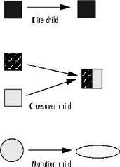
The genetic algorithm creates three types of children for the next generation:
-
Eliteare the individuals in the current generation with the best fitness values. These individuals automatically survive to the next generation.
-
Crossover are created by combining the vectors of a pair of parents.
-
Mutation children are created by introducing random changes, or mutations, to a single parent.
The following schematic diagram illustrates the three types of children.
Flowchart :
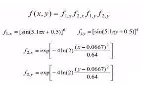
function [f] = stalagmite(input_vector);
x = input_vector(1);
y = input_vector(2);
f1_x = (sin(5.1*pi*x+0.5)).^6;
f1_y = (sin(5.1*pi*y+0.5)).^6;
t1 = (x-0.0667).^2/(0.64);
f2_x = exp(-4.*log(2)*t1);
t2 = (y-0.0667).^2/(0.64);
f2_y = exp(-4.*log(2)*t2);
f = -(f1_x.*f2_x.*f1_y.*f2_y);
- First a variable 'f' is defined for the slagmite function.
- Stalagmite function takes the values of 'input vector' and calculates the value of 'f'.
- The function 'f' deals with two variables (x ,y).
- The terms involved in the formula are [f1_x, f2_x, f1_y, f2_y].
- x is stored in an array called 'input vector(1)'.
- y is stored in an array called 'input vector(2)'.
- The formula is written in syntax for every term.
- And all the term are multiplied and a '-' sign is given in the syntax to make the plot in positive x-axis.
Explanation of Code :
clear all
close all
clc
Clear all - Clear all command is used to clear all the previous running function in the workspace.
Close all - Close all command is used to close all the previous running plots and graphs running in the background.
clc - clc command is used to clear the workspace.
%Defining our search space.
x = linspace(0,0.6,150)
y = linspace(0,0.6,150)


%Creating a 2D mesh.
[X,Y] = meshgrid(x,y);
For defining the search space :
- We are specifying the x-axis to plot the graph from 0 - 0.6.
- We are specifying the y-axis to plot the graph from 0 - 0.6.
For creating a 2D mesh :
- We use the 'meshgrid' command.
- meshgrid(x,y) returns 2-D grid coordinates based on the coordinates contained in vectors x and
y.Xis a matrix where each row is a copy ofx, andYis a matrix where each column is a copy ofy. The grid represented by the coordinatesXandYhas length(y) rows and length(x) columns.
%evaluating the stalagmite function.

for  i = 1:length(X);
   for j = 1:length(Y);
    input_vector(1) = X(i,j);
    input_vector(2) = Y(i,j);
    f(i,j) = stalagmite(input_vector);

   end
end
For evaluating the stalagmite function
We create a 'for loop' :
- 'i' is a variable used to define the values for the whole length of x.
- 'j' is a variable used to define the values for the whole length of y.
- 'input_vector' is a row vector i.e it has 2 columns.
- We take the two values of x and y and put them in an array called the 'input_vector'.
- Now the function stalagmite takes in the input vector and calculates the value of 'f'.
- 'end' command is used to finish the for loop.
Plot :
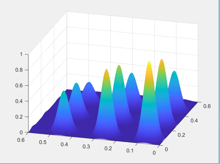
The above figure shows the plot for mathematical stalagmite function for this case.
CASE 1 :
UNBOUNDED BEHAVIOUR :
% UNBOUNDED BEHAVIOUR.
% study 1 statistical behaviour.
% calculating the study time with tic and toc command.

tic
num_cases = 50
for  i = 1:num_cases;
    [inputs, fopt(i)] = ga(@getstalagmite,2);
    Xopt(i)=inputs(1);
    Yopt(i)=inputs(2);

end
study_time1 = toc

%plotting the graph.
figure(1);
subplot(2,1,1)
surf(X,Y,f);
hold on
shading interp
plot3(Xopt,Yopt,-fopt,'marker','o','markersize',5,'markerfacecolor','r');
xlabel('x')
ylabel('y')
grid on
subplot(2,1,2)
plot(-fopt);
xlabel('iterations')
ylabel('function min value')
- To calculate the study time we use the tic and toc command.
- 'tic' works with the 'toc' function to measure elapsed time. The 'tic' function records the current time, and the 'toc' function uses the recorded value to calculate the elapsed time.
- The command 'num_cases' instructs the matlab to run the function for 50 iterations and evaluate the fitness.
- Then we create a 'for loop' with a variable 'i'.
- 'i = 1:num_cases' - is the variable command which stores the values for each 50 iteration of fitness for this function.
- '[inputs, fopt(i)]' - calculates the optimum value of 'f' for the specific range of the function.
- 'getstalagmite' - is the command which is used to call the stalagmite function which we have saved to make the coding easier.
- xopt(i) takes the input for 1st variable.
- yopt(i) takes the input for 2nd variable.
- we 'end' the for loop.
Plotting the graph :
- For the figure(1) we use subplot command.
- 'subplot(2,1,1)' divides the current figure into an 2-by-1 grid and creates axes in the position specified by 1. If axes exist in the specified position, then this command makes the axes the current axes.
- 'surf(X,Y, f)' creates a three-dimensional surface plot, which is a three-dimensional surface that has solid edge colors and solid face colors. The function plots the values in matrix 'f' as heights above a grid in the X-Y plane defined by X and Y. The color of the surface varies according to the heights specified by f.
- 'hold on' command is used to keep both the plots.
- As we are dealing with 3-d plot, we use the 'plot3' command to make the 3-D array of (Xopt,Yopy,fopt), with a marker 'o' markersize 5 and color red.
- The '-' sign is given to make the plot on a positive x- axis, for our own convenience.
- 'xlabel' is given the name x-axis.
- 'ylabel' is given the name y-axis.
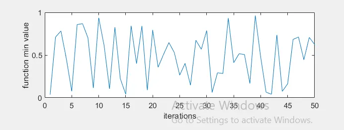
- 'plot(-fopt)' plots the graph for the different value of the fitness of the stalagmite function.
- xlabel is given the name 'iterations'.
- ylabel is given the name 'function min value'.
Plots :

Result :
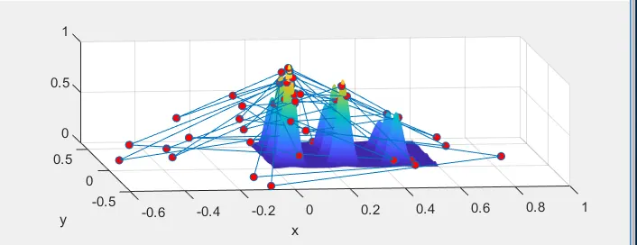
- As we can see from the above plots the result is not very clear hence optimization is not accurate.
- Hence, we need to perform the function with bounded parameters.
- Study time for the first study behaviour is 4.3335.
CASE 2 :
BOUNDED BEHAVIOUR :
%BOUNDED BEHAVIOUR
%study 2 statistical behaviour with lower bound and upper bound.

num_cases = 50
tic
for l = 1:num_cases;
    [inputs,fopt(l)] = ga(@getstalagmite,2,[],[],[],[],[0;0],[0.6;0.6]); % calculating the each value with boundation
    Xopt(l) = inputs(1);
    Yopt(l) = inputs(2);

end
study_time2 = toc

%plotting the graph
figure(2)
subplot(2,1,1);
hold on
surf(X,Y,f);
plot3(Xopt,Yopt,-fopt,'marker','o','markersize',5,'markerfacecolor','r');
xlabel('x')
ylabel('y')
grid on
subplot(2,1,2);
plot(-fopt);
xlabel('iterations')
ylabel('function min value')
- To calculate the study time we use the tic and toc command.
- 'tic' works with the 'toc' function to measure elapsed time. The 'tic' function records the current time, and the 'toc' function uses the recorded value to calculate the elapsed time.
- The command 'num_cases' instructs the matlab to run the function for 50 iterations and evaluate the fitness.
- Then we create a 'for loop' with a variable 'l'.
- 'l = 1:num_cases' - is the variable command which stores the values for each 50 iteration of fitness for this function.
- '[inputs, fopt(l)]' - calculates the optimum value of 'f' for the specific range of the function.
- 'getstalagmite' - is the command which is used to call the stalagmite function which we have saved to make the coding easier.
- xopt(l) takes the input for 1st variable.
- yopt(l) takes the input for 2nd variable.
- we 'end' the for loop.
Explanation of genetic algorithm(ga) syntax :
x = ga(fun,nvars,A,b,Aeq,beq,lb,ub)
fun - fitnesss function.
nvars - Number of design variables.
A [] = A matrix for linear inequality constraints.
b [] = b vector for linear inequality constraints.
Aeq [] = Aeq matrix for linear equality constraints.
beq [] = beq vector for linear equality constraints.
lb = lower bound on x.
ub = upper bound on x.
Plotting the graph :
- For the figure(1) we use subplot command.
- 'subplot(2,1,1)' divides the current figure into an 2-by-1 grid and creates axes in the position specified by 1. If axes exist in the specified position, then this command makes the axes the current axes.
- 'surf(X,Y, f)' creates a three-dimensional surface plot, which is a three-dimensional surface that has solid edge colors and solid face colors. The function plots the values in matrix 'f' as heights above a grid in the X-Y plane defined by X and Y. The color of the surface varies according to the heights specified by f.
- 'hold on' command is used to keep both the plots.
- As we are dealing with 3-d plot, we use the 'plot3' command to make the 3-D array of (Xopt,Yopy,fopt), with a marker 'o' markersize 5 and color red.
- The '-' sign is given to make the plot on a positive x- axis, for our own convenience.
- 'xlabel' is given the name x-axis.
- 'ylabel' is given the name y-axis.
- 'plot(-fopt)' plots the graph for the different value of the fitness of the stalagmite function.
- xlabel is given the name 'iterations'.
- ylabel is given the name 'function min value'.
PLOTS :
Result :
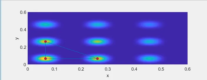
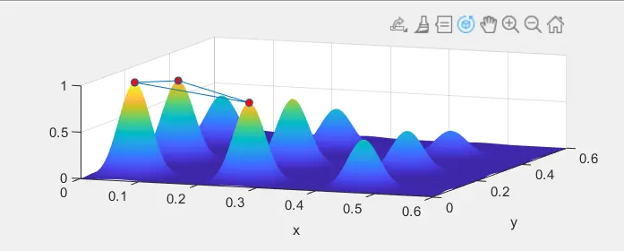
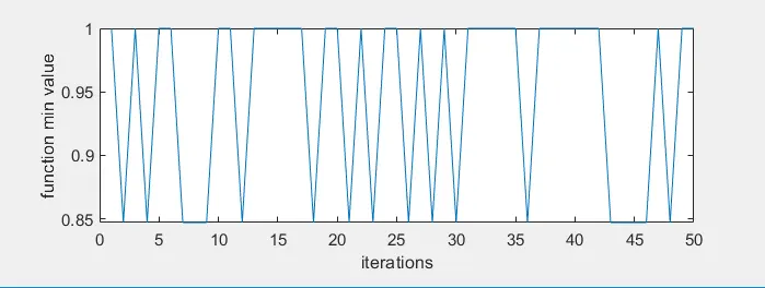
- It can be easily understood that by giving a boundary condition the optimization is much accurate and variation decreased drastically.
- However we need to specify a population size to the study for more accurate result.
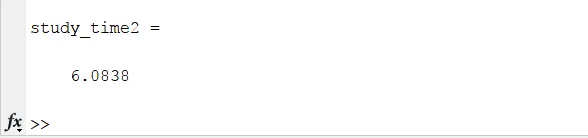
- The study time is 6.0838.
CASE 3 :
STUDY WITH POPULATION SIZE :
%STUDY WITH INCREASE IN POPULATION.
%study 3 increasing the iterations of the ga function.

options = optimoptions('ga');
options = optimoptions(options,'populationsize',170)

num_cases = 50
for k = 1:num_cases;
    [inputs fopt(k)] = ga(@getstalagmite,2,[],[],[],[],[0;0],[0.6;0.6],[],[],options);
    Xopt(k) = inputs(1)
    Yopt(k) = inputs(2)

end
study_time3 = toc

figure(3)
subplot(2,1,1)
hold on
surf(X,Y,f)
plot3(Xopt,Yopt,-fopt,'marker','o','markersize',5,'markerfacecolor','r')
xlabel('x')
ylabel('y')
shading interp
grid on
subplot(2,1,2)
plot(-fopt)
xlabel('iterations')
ylabel('function min value')
- To calculate the study time we use the tic and toc command.
- 'tic' works with the 'toc' function to measure elapsed time. The 'tic' function records the current time, and the 'toc' function uses the recorded value to calculate the elapsed time.
- The command 'num_cases' instructs the matlab to run the function for 50 iterations and evaluate the fitness.
- Then we create a 'for loop' with a variable 'k'.
- 'k= 1:num_cases' - is the variable command which stores the values for each 50 iteration of fitness for this function.
- '[inputs, fopt(k)]' - calculates the optimum value of 'f' for the specific range of the function.
- 'getstalagmite' - is the command which is used to call the stalagmite function which we have saved to make the coding easier.
- xopt(k) takes the input for 1st variable.
- yopt(k) takes the input for 2nd variable.
- we 'end' the for loop.
Explanation of genetic algorithm(ga) syntax :
x = ga(fun,nvars,A,b,[],[],lb,ub,nonlcon,IntCon,options)
fun - fitnesss function.
nvars - Number of design variables.
A [] = A matrix for linear inequality constraints.
b [] = b vector for linear inequality constraints.
Aeq [] = Aeq matrix for linear equality constraints.
beq [] = beq vector for linear equality constraints.
lb = lower bound on x.
ub = upper bound on x.
nonlcon [] = non linear constraint function.
Intcon [] = interger constraint function.
options - Options created using optimoptions or an options structure
Plotting the graph :
- For the figure(1) we use subplot command.
- 'subplot(2,1,1)' divides the current figure into an 2-by-1 grid and creates axes in the position specified by 1. If axes exist in the specified position, then this command makes the axes the current axes.
- 'surf(X,Y, f)' creates a three-dimensional surface plot, which is a three-dimensional surface that has solid edge colors and solid face colors. The function plots the values in matrix 'f' as heights above a grid in the X-Y plane defined by X and Y. The color of the surface varies according to the heights specified by f.
- 'hold on' command is used to keep both the plots.
- As we are dealing with 3-d plot, we use the 'plot3' command to make the 3-D array of (Xopt,Yopy,fopt), with a marker 'o' markersize 5 and color red.
- The '-' sign is given to make the plot on a positive x- axis, for our own convenience.
- 'xlabel' is given the name x-axis.
- 'ylabel' is given the name y-axis.
- 'plot(-fopt)' plots the graph for the different value of the fitness of the stalagmite function.
- xlabel is given the name 'iterations'.
- ylabel is given the name 'function min value'.
Plots :
Result :
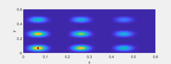
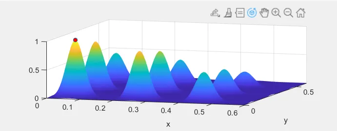
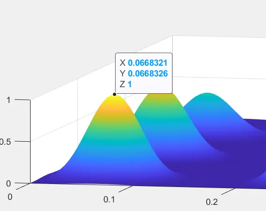
- Here the red point gives us the global maxima at a population size of 170.
- The optimum value for x = 0.0668321.
- The optimum value for y= 0.0668326.
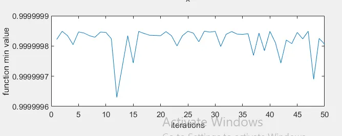
- And the value of f =1 , which is ideal for optimum condition.
Genetic Algorithm Code :
clear all
close all
clc

%Defining our search space.
x = linspace(0,0.6,150);
y = linspace(0,0.6,150);


%Creating a 2D mesh.
[X,Y] = meshgrid(x,y);

%evaluating the stalagmite function.

for  i = 1:length(X);
   for j = 1:length(Y);
    input_vector(1) = X(i,j);
    input_vector(2) = Y(i,j);
    f(i,j) = stalagmite(input_vector);

   end
end

surf(X,Y,f) %to generate the surface.
shading interp % to remove the meshgrid lines.


% UNBOUNDED BEHAVIOUR.
% study 1 statistical behaviour.
% calculating the study time with tic and toc command.

tic
num_cases = 50
for  i = 1:num_cases;
    [inputs, fopt(i)] = ga(@getstalagmite,2);
    Xopt(i)=inputs(1);
    Yopt(i)=inputs(2);

end
study_time1 = toc

%plotting the graph.
figure(1);
subplot(2,1,1)
surf(X,Y,f);
hold on
shading interp
plot3(Xopt,Yopt,-fopt,'marker','o','markersize',5,'markerfacecolor','r');
xlabel('x')
ylabel('y')
grid on
subplot(2,1,2)
plot(-fopt);
xlabel('iterations')
ylabel('function min value')


%BOUNDED BEHAVIOUR
%study 2 statistical behaviour with lower bound and upper bound.

num_cases = 50
tic
for l = 1:num_cases;
    [inputs,fopt(l)] = ga(@getstalagmite,2,[],[],[],[],[0;0],[0.6;0.6]); % calculating the each value with boundation
    Xopt(l) = inputs(1);
    Yopt(l) = inputs(2);

end
study_time2 = toc

%plotting the graph
figure(2)
subplot(2,1,1);
hold on
surf(X,Y,f);
plot3(Xopt,Yopt,-fopt,'marker','o','markersize',5,'markerfacecolor','r');
xlabel('x')
ylabel('y')
grid on
shading interp
subplot(2,1,2);
plot(-fopt);
xlabel('iterations')
ylabel('function min value')
%


%STUDY WITH INCREASE IN POPULATION.
%study 3 increasing the iterations of the ga function.

options = optimoptions('ga');
options = optimoptions(options,'populationsize',170)

num_cases = 50
for k = 1:num_cases;
    [inputs fopt(k)] = ga(@getstalagmite,2,[],[],[],[],[0;0],[0.6;0.6],[],[],options);
    Xopt(k) = inputs(1)
    Yopt(k) = inputs(2)

end
study_time3 = toc

figure(3)
subplot(2,1,1)
hold on
surf(X,Y,f)
plot3(Xopt,Yopt,-fopt,'marker','o','markersize',5,'markerfacecolor','r')
xlabel('x')
ylabel('y')
shading interp
grid on
subplot(2,1,2)
plot(-fopt)
xlabel('iterations')
ylabel('function min value')
Error :
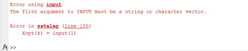
1. 'String Error' :
Solution :
- While defining the optimum values we used the 'input' command which bassically displays the text in prompt.
- But for this function we needed a string to read the values.
- Hence, the error was evident.
- we corrected the issue by including a string to the function with 'inputs' command.
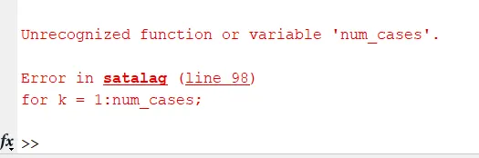
2. 'num_cases' Error' :
Solution :
- While defining the 'for loop' we made the mistake of not defining the number of cases to be calculated.
- The number of cases we defined was 50.
- Hence, the error was corrected.
References :
- https://in.mathworks.com/help/gads/ga.html#d122e38546
- https://en.wikipedia.org/wiki/Genetic_algorithm
- https://skill-lync.com/projects/week-4-genetic-algorithm-33