Week 3 - Solving second order ODEs

AIM : Write a program in Matlab that will simulate the pendulum motion, to describe the transient behavior of a system.

Governing Equation:

An ordinary differential equation (ODE) is a differential equation containing one or more functions of one independent variable and the derivatives of those functions. The term ordinary is used in contrast with the term partial differential equation which may be with respect to more than one independent variable.

The equation we are dealing with are:

In the above equation

g = gravity in m/s2,

L = length of the pendulum in m,

m = mass of the ball in kg,

b=damping coefficient.

`d^2/dt^2`(`theta`)+b/m *`d/dt`(`theta`)+g/l*sin(`theta`) = 0

Lets say,

`theta`=`theta1`

and

`d/dt`(`theta`)=`d/dt`(`theta1`)=`theta2`

Now substituting `theta1`and `theta2` values we get:

``d^2/dt^2`(`theta1`)+b/m`d/dt`(`theta1`)+g/l * sin(`theta1`)=0

`d^2/dt^2`(`theta1`)+b/m*(`theta2`)+g/l*sin(`theta1`) =0

`d/dt`(`theta2`)+b/m *(`theta2`)+g/l* sin (`theta1`) = 0

We arranged the equation in a column matrix to solve the equation.

`d/dt``((theta),(theta1))`= `[[theta2,0],[-b/mtheta2-g/lsintheta1]]`

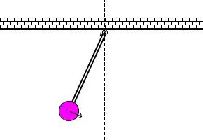
A simple pendulum consists of a bob hanging from a string fixed to a pivot joint with a base.

The way the pendulum moves depends on the Newtons second law. When this law is written down, we get a second order Ordinary Differential Equation that describes the position of the "ball" w.r.t time.

There are two dominant forces acting upon a pendulum bob at all times during the course of its motion.

1. There is the force of gravity that acts downward upon the bob. It results from the Earth's mass attracting the mass of the bob.
2. And there is a tension force acting upward and towards the pivot point of the pendulum.

OBJECTIVE :

• Create an image that represents the position of the pendulum.
• Use the marker command to create a sphere.
• usage the movie command create an animation.

Explanation of function:

Functions allows us to reuse sequences of commands by storing them in program files. Functions are the simplest type of program, since they store commands exactly as you would type them at the command line.

Functions provide more flexibility, primarily because we can pass input values and return output values.

function [dtheta_dt] = ode_func(t,theta,b,g,l,m);

theta1 = theta(1)
theta2 = theta(2)

dtheta1_dt = theta2;
dtheta2_dt = [-(b/m)*(theta2)-(g/l)*sin(theta1)];
dtheta_dt = [dtheta1_dt;dtheta2_dt];
    
end

First step:

A variable (`d/dt``theta`) is given a function name 'ode_func'.

The ode_func has been given some specific parameters such as

t = integration time.

theta = subtended angle by pendulum.

b = damping coefficient.

l = length.

m = masss.

2nd step:

theta1 is given a name theta(1).

theta2 is given a name theta(2).

3rd step:

The terms are written down in syntax:

`d/dt`(`theta1`) = `theta2`

`d/dt`(`theta2`) = -b/m*(`theta2`)-g/l*sin(`theta1`)

4th step:

The equation is given a matrix form and a semicolon is provided to make a column matrix.

`d/dt` = makes a column matrix between `d/dt`(`theta1`) and `d/dt`(`theta2`) to perform the matrix operation, so that the calculation is easier.

Explanation of code :

%input parameters
b = 0.05;
g = 9.81;
l = 1;
m = 0.1;

theta_0 = [0;5];

First,

we defined the input parameters where

acceleration due to gravity(g) = 9.81m/s

length(l) = 1m

mass(m) = 0.1m

damping coefficient(b) = 0.05

theta_0 = [0;5] is defined as

1. Initial velocity is 0.
2. Initial displacement is 5.

%time span
t_span = linspace(0,20,500);

Next,

The time span of the pendulum is defined where the pendulum motion will operate from (0-20) seconds.

And it will take 500 values in between to give us the necessary output.

%solve for ODE

figure(1)
[t,results] = ode45(@(t,theta) ode_func(t,theta,b,g,l,m),t_span,theta_0);
theta = results(:,1);

Ode45 is a function in matlab that solves ordinary or partial differential equations using a numerical method. The numerical method in question here is the 4th order Runge Kutta method.

ode45 solves for the specific integration time and different values of theta.

Hence, it gives two column of results for velocity and displacement.

ode_func is a function we have made to define the various parameters such as (t,theta,b,g,l,m) such that the code gets easy to solve.

t_span is the time span for pendulum to run for a specific time.

theta_0 is the intial conditions for velocity and displacement.

Here theta considers the first column of the results i.e velocity.

subplot(2,1,2)
plot(t,results(:,1),'linewidth',2,'color','b')
xlabel('time');
ylabel('angular velocity');
grid on

Subplot :

This command divides the current figure into an m-by-n grid and creates axes in the position specified. Matlab numbers subplot positions by row. The first subplot is the first column of the first row, the second subplot is the second column of the first row, and so on. If axes exist in the specified position, then this command makes the axes the current axes.

plot(t,results) -

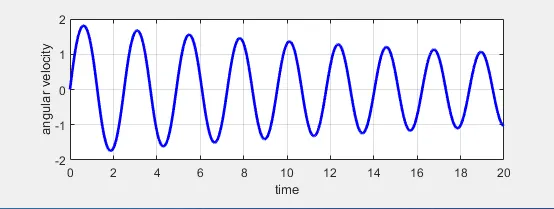
This command plots the graphs between time and angular velocity for each iteration of the pendulum.

The initial condition of the graph is given 0 m/s, hence it starts the graph from 0 m/s.

xlabel('time') - means the x axis is given the name time.

ylabel('angular velocity') - means the y axis is given the name angular velocity.

grid on - 'grid on' displays the major grid lines for the current axes, major grid lines extend from each tick mark.

subplot(2,1,1)
plot(t,results(:,2),'linewidth',2,'color','m')
xlabel('time');
ylabel('displacement');
grid on

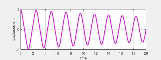
'Plot' command makes a graph between displacemet vs time for each iteration of the pendulum.

The initial condition of the graph is 5m/s, hence it starts the graph from 5 m/s.

xlabel('time') - The x-axis is given the name time.

ylabel('displacement') - The y-axis is given the name displacement.

grid on - 'grid on' displays the major grid lines for the current axes, major grid lines extend from each tick mark.

For loop :

A 'for loop' is a repetition control structure that allows you to efficiently write a loop that needs to execute a specific number of times. The syntax of 'for loop' for this function is as following:

ct = 1;
for i = 1:length(theta);
    Theta = theta(i);
     % initial position
     x = 0;
     y = 0;
     x1 = l*sin(Theta);
     y1 = -l*cos(Theta);
     figure(2)
     %base
     plot([-1 1],[0 0],'linewidth',3,'color','k');
     hold on;
     %string:
     plot([x x1],[y y1],'linewidth',2,'color','r');
     %bob of pendulumn
     plot(x1,y1,'marker','o','markersize',40,'markerfacecolor','b');
     hold off
     axis([-1.5 1.5 -2 1]);
      
    M(ct) = getframe(gcf);
    ct = ct+1;
 end

First, we give a counter variable(ct) for the first frame.

Then we took a variable named (i) for the loop, the value of the loop ranges from 1 to the length of theta, where theta represents the values of angular velocity from the results column.

Theta = theta(i) considers every value of angular velocity.

The initial position is given by :

x = 0 for x co-ordinate.

y = 0 for y co-ordinate.

and,

x1 = l*sin(theta)

y1 = -l*cos(theta)

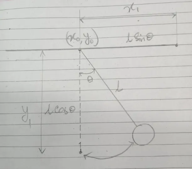
plot([-1 1],[0 0],'linewidth',2,'color','k');

This is the command to plot the base line of pendulum from -1 to 1 along the x-axis and (0,0) the midpoint of the base of the pendulum with linewidth 2 and color black.

plot([x x1] [y y1],'linewidth',2,'color','r');

This command is to plot the line of pendulum from (x to x1) along x-axis and (y to y1) along y-axis, with linewidth 2 and color red.

plot(x1,y1,'marker','o','markersize',40,'markerfacecolor','b');

This command is given to draw the bob of the pendulum of specific size.

'marker' - Adding markers to a line plot can be a useful way to distinguish multiple lines or to highlight particular data points.

A markersize of 40 is used.

and markerfacecolor of blue is used to draw the bob of pendulum.

axis[-1.5 1.5 -2 1]

The axis is drawn from (-1.5 to 1.5) along x-axis and (-2 to 1) along y-axis for the animation of the pendulum.

• The M command is used as a array.
• A counter variable (ct) is used to define each and every frame.
• 'getframe' is a command used for current figure window.
• 'movie(m)' command is used to generate the movie with all the frame.
• [ct=ct+1] is used to add the next frame with each individual iterations

%  command for animation
 movie(M)
 videofile = VideoWriter('pendulumn_motion.avi','uncompressed AVI');
 open(videofile);
 writeVideo(videofile,M);
 close(videofile);

• 'movie(m)' command is used to generate the movie with all the frame.
• 'videofile' is a comand used to create the videowriter.
• '(pendulumn_motion.avi)' is the file name that is used to define the file.
• 'open(videofile)' is the command used to open the file.
• 'writeVideo(videofile,M)' is the command used to write the video file.
• 'close(videofile)' is used to close the function.

CODE :

%input parameters
b = 0.05;
g = 9.81;
l = 1;
m = 1;

theta_0 = [0;5];

%time span
t_span = linspace(0,20,500);

%solve for ODE

figure(1)
[t,results] = ode45(@(t,theta) ode_func(t,theta,b,g,l,m),t_span,theta_0);
theta = results(:,1);
hold on

subplot(2,1,2)
plot(t,results(:,1),'linewidth',2,'color','b')
xlabel('time');
ylabel('angular velocity');
grid on

subplot(2,1,1)
plot(t,results(:,2),'linewidth',2,'color','m')
xlabel('time');
ylabel('displacement');
grid on

ct = 1;
for i = 1:length(Theta);
    Theta = theta(i);
     % initial position
     x = 0;
     y = 0;
     x1 = l*sin(Theta);
     y1 = -l*cos(Theta);
     figure(2)
     %base
     plot([-1 1],[0 0],'linewidth',3,'color','k');
     hold on;
     %string
     plot([x x1],[y y1],'linewidth',2,'color','r');
     %bob of pendulumn
     plot(x1,y1,'marker','o','markersize',40,'markerfacecolor','b');
     hold off
     axis([-1.5 1.5 -2 1]);
      
    M(ct) = getframe(gcf);
    ct = ct+1
 end
 
% command for animation
 movie(M);
 videofile = VideoWriter('pendulumn_motion.avi','uncompressed AVI');
 open(videofile);
 writeVideo(videofile,M);
 close(videofile);

PLOTS:

Angular velocity vs Time

Displacement vs Time

ERROR :

1. 'Bracket' Error :

• Generally square brackets are used for array construction and concatenation.
• Empty matrix and array element deletion.
• Multiple output argument assignment.

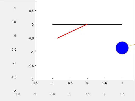
Solution:

While giving the command to plot the bob of pendulum we used square brackets, as the co-ordinates were not an array of matrix for this specific plot, it gave us a hapazard animation.

using the correct parentheses we corrected the issue.2

2. 'getframe error' :

• 'getframe' captures the current axes as it appears on the screen as a movie frame.
• 'getframe' captures the axes at the same size that it appears on the screen. It does not capture tick labels or other content outside the axes outline.

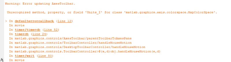
Solution:

We made a mistake of not defining the 'getframe' command as a result of which the figure was absent from the present window and it gave us an error.

We corrected the mistake by ' M(ct) = getframe(gcf)' command.\

conclusion :

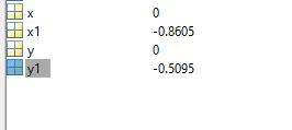
The (x,x1)and (y,y1) values are shown as above.

Animation :

https://www.youtube.com/watch?v=kKR4xHt6e5I

References:

• https://en.wikipedia.org/wiki/Pendulum
• https://www.khanacademy.org/computing/computer-programming/programming-natural-simulations/programming-oscillations/a/trig-and-forces-the-pendulum